Data Sources

Open Repositories

Data Portals

Pages Listing Data Sets

  • Wikipedia: List of datasets for machine learning research
  • Quora: Where can I find large datasets open to the public?
  • Reddit: r/datasets

References

Short Codes

These are short-hand codes to make it easier to quickly refer to sources.

  • [HOML]: Hands-On Machine Learning with Scikit-Learn and TensorFlow

Bibliography

  • Géron, Aurélien. Hands-on Machine Learning with Scikit-Learn and TensorFlow: Concepts, Tools, and Techniques to Build Intelligent Systems. First edition. Beijing Boston Farnham: O’Reilly, 2017.

California Housing Prices

Introduction

This is an introductory regression problem that uses California housing data from the 1990 census. There's a description of the original data here, but we're using a slightly altered dataset that's on github (and appears to be mirrored on kaggle). The problem here is to create a model that will predict the median housing value for a census block group (called "district" in the dataset) given the other attributes. The original data is also available from sklearn so I'm going to take advantage of that to get the description and do a double-check of the model.

Imports

These are the dependencies for this problem.

# python standard library
import os
import tarfile
import warnings
warnings.filterwarnings("ignore", message="numpy.dtype size changed")
from http import HTTPStatus

# from pypi
import matplotlib
import pandas
import requests
import seaborn
from sklearn.datasets import fetch_california_housing
from tabulate import tabulate

Constants

These are convenience holders for strings and other constants so they don't get scattered all over the place.

class Data:
    source_slug = "../data/california-housing-prices/"
    target_slug = "../data_temp/california-housing-prices/"
    url = "https://github.com/ageron/handson-ml/raw/master/datasets/housing/housing.tgz"
    source = source_slug + "housing.tgz"
    target = target_slug + "housing.csv"
    chunk_size = 128

The Data

We'll grab the data from github, extract it (it's a tgz compressed tarfile), then make a pandas data frame from it. I'll also download the sklearn version.

Downloading the sklearn dataset

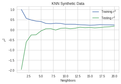
sklearn_housing_bunch = fetch_california_housing("~/data/sklearn_datasets/")
Downloading Cal. housing from https://ndownloader.figshare.com/files/5976036 to /home/brunhilde/data/sklearn_datasets/
print(sklearn_housing_bunch.DESCR)
California housing dataset.

The original database is available from StatLib

    http://lib.stat.cmu.edu/datasets/

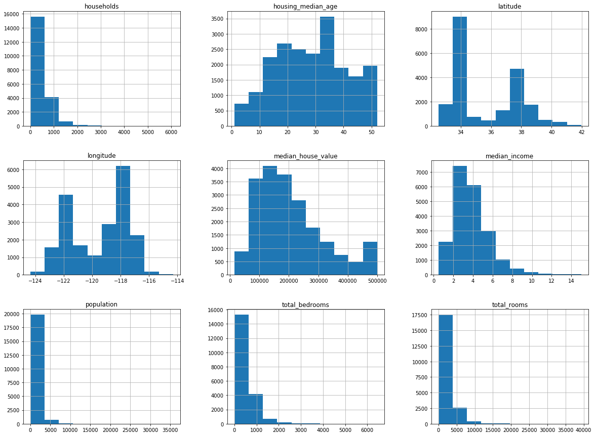
The data contains 20,640 observations on 9 variables.

This dataset contains the average house value as target variable
and the following input variables (features): average income,
housing average age, average rooms, average bedrooms, population,
average occupation, latitude, and longitude in that order.

References
----------

Pace, R. Kelley and Ronald Barry, Sparse Spatial Autoregressions,
Statistics and Probability Letters, 33 (1997) 291-297.


print(sklearn_housing_bunch.feature_names)

['MedInc', 'HouseAge', 'AveRooms', 'AveBedrms', 'Population', 'AveOccup', 'Latitude', 'Longitude']

Now I'll convert it to a Pandas DataFrame.

sklearn_housing = pandas.DataFrame(sklearn_housing_bunch.data,
				   columns=sklearn_housing_bunch.feature_names)
             MedInc      HouseAge      AveRooms     AveBedrms    Population  \
count  20640.000000  20640.000000  20640.000000  20640.000000  20640.000000   
mean       3.870671     28.639486      5.429000      1.096675   1425.476744   
std        1.899822     12.585558      2.474173      0.473911   1132.462122   
min        0.499900      1.000000      0.846154      0.333333      3.000000   
25%        2.563400     18.000000      4.440716      1.006079    787.000000   
50%        3.534800     29.000000      5.229129      1.048780   1166.000000   
75%        4.743250     37.000000      6.052381      1.099526   1725.000000   
max       15.000100     52.000000    141.909091     34.066667  35682.000000   

           AveOccup      Latitude     Longitude  
count  20640.000000  20640.000000  20640.000000  
mean       3.070655     35.631861   -119.569704  
std       10.386050      2.135952      2.003532  
min        0.692308     32.540000   -124.350000  
25%        2.429741     33.930000   -121.800000  
50%        2.818116     34.260000   -118.490000  
75%        3.282261     37.710000   -118.010000  
max     1243.333333     41.950000   -114.310000  

Downloading and uncompressing the data

def get_data():
    """Gets the data from github and uncompresses it"""
    if os.path.exists(Data.target):
	return

    os.makedirs(Data.target_slug, exist_ok=True)
    os.makedirs(Data.source_slug, exist_ok=True)
    response = requests.get(Data.url, stream=True)
    assert response.status_code == HTTPStatus.OK
    with open(Data.source, "wb") as writer:
	for chunk in response.iter_content(chunk_size=Data.chunk_size):
	    writer.write(chunk)
    assert os.path.exists(Data.source)
    compressed = tarfile.open(Data.source)
    compressed.extractall(Data.target_slug)
    compressed.close()
    assert os.path.exists(Data.target)
    return

Contents of ../data_temp/california-housing-prices/:

  • housing.csv

Building the dataframe

housing = pandas.read_csv(Data.target)
<class 'pandas.core.frame.DataFrame'>
RangeIndex: 20640 entries, 0 to 20639
Data columns (total 10 columns):
longitude             20640 non-null float64
latitude              20640 non-null float64
housing_median_age    20640 non-null float64
total_rooms           20640 non-null float64
total_bedrooms        20433 non-null float64
population            20640 non-null float64
households            20640 non-null float64
median_income         20640 non-null float64
median_house_value    20640 non-null float64
ocean_proximity       20640 non-null object
dtypes: float64(9), object(1)
memory usage: 1.6+ MB
None

Comparison to Sklearn

The dataset seems to differ somewhat from the sklearn description. Instead of total_rooms they have AveRooms, for instance. Is this just a problem of names?

print(sklearn_housing.AveRooms.head())

0 6.984127 1 6.238137 2 8.288136 3 5.817352 4 6.281853 Name: AveRooms, dtype: float64

print(housing.total_rooms.head())

0 880.0 1 7099.0 2 1467.0 3 1274.0 4 1627.0 Name: total_rooms, dtype: float64

So they are different. Let's see if you can get the sklearn values from the original data set.

print((housing.total_rooms/housing.households).head())

0 6.984127 1 6.238137 2 8.288136 3 5.817352 4 6.281853 dtype: float64

It looks like the sklearn values are (in some cases) calculated values derived from the original. It makes sense that they changed some of the things (total number of rooms only makes sense if there is the same number of households in each district, for instance), but it would have been better if they documented the changes they made and why they changed it.

Inspecting the Data

If you look at the total_bedrooms count you'll see that it only has 20,433 non-null values, while the rest of the columns have 20,640 values. These were removed to allow experimenting with missing data. The original dataset that was collected for the census had all the values.

Column Has Missing Values
longitude False
latitude False
housing_median_age False
total_rooms False
total_bedrooms True
population False
households False
median_income False
median_house_value False
ocean_proximity False

It looks like total_bedrooms is the only column where there's missing data.

Rows Columns
20640 10

I'll print the median for each column except the last (since it's non-numeric).

longitude latitude housing_median_age total_rooms
-118.49 34.26 29.00 2127.00
total_bedrooms population households median_income median_house_value
435.00 1166.00 409.00 3.53 179700.00

Here's the description for the ocean_proximity variable Looking at the median_income you can see that it isn't income in dollars.

Statistic Value
count 20640
unique 5
top <1H OCEAN
freq 9136

It looks like the most common house location is less than an hour from the ocean.

print(
    "{:.2f}".format(
	ocean_proximity_description.loc["freq"]/ocean_proximity_description.loc["count"]))

0.44

Which makes up about forty-four percent of all the houses. Here are all the ocean_proximity values.

ocean_proximity.png

Proximity Count Percentage
<1H OCEAN 9136 44.2636
INLAND 6551 31.7393
NEAR OCEAN 2658 12.8779
NEAR BAY 2290 11.095
ISLAND 5 0.0242248

housing_histogram.png

If you look at the median income plot you can see that it goes from 0 to 15. It turns out that the incomes were re-scaled and limited to the 0.5 to 15 range. The median age and value were also capped, possibly affecting our price predictions.

References

  • Géron, Aurélien. Hands-on Machine Learning with Scikit-Learn and TensorFlow: Concepts, Tools, and Techniques to Build Intelligent Systems. First edition. Beijing Boston Farnham: O’Reilly, 2017.

Decision Tree Classification

1 Imports

import graphviz
from sklearn.tree import (
    DecisionTreeClassifier,
    export_graphviz,
    )
from sklearn.model_selection import train_test_split
from sklearn.datasets import load_breast_cancer
% matplotlib inline

2 The Data

cancer = load_breast_cancer()
print(cancer.keys())
dict_keys(['DESCR', 'target_names', 'data', 'feature_names', 'target'])
X_train, X_test, y_train, y_test = train_test_split(cancer.data,
                                                    cancer.target,
                                                    stratify=cancer.target)

3 The Model

def build_tree(max_depth=None):
    tree = DecisionTreeClassifier(max_depth=max_depth)
    tree.fit(X_train, y_train)
    print("Max Depth: {0}".format(max_depth))
    print("Training Accuracy: {0:.2f}".format(tree.score(X_train, y_train)))
    print("Testing Accuracy: {0:.2f}".format(tree.score(X_test, y_test)))
    print()
    return

build_tree()
Max Depth: None
Training Accuracy: 1.00
Testing Accuracy: 0.93

It looks like the tree is overfitting the training data. This is because the default tree will have leaf nodes that match each case in the training data set. Limiting the depth of the tree will help with this.

for depth in range(1, 5):
    build_tree(depth)
Max Depth: 1
Training Accuracy: 0.92
Testing Accuracy: 0.90

Max Depth: 2
Training Accuracy: 0.95
Testing Accuracy: 0.92

Max Depth: 3
Training Accuracy: 0.96
Testing Accuracy: 0.92

Max Depth: 4
Training Accuracy: 0.98
Testing Accuracy: 0.91

The book was able to get 95% accuracy for the training data, although I don't seem to be able to do better than 92%.

4 Visualizing The Tree

tree = DecisionTreeClassifier(max_depth=3)
tree.fit(X_train, y_train)
export_graphviz(tree, out_file="tree.dot", class_names=cancer.target_names,
                feature_names=cancer.feature_names, impurity=False,
                filled=True)
with open("tree.dot") as reader:
    dot_file = reader.read()

graphviz.Source(dot_file, format="png").render("tree")
tree.png

Naive Bayes Classification

1 Imports

from sklearn.naive_bayes import GaussianNB
from sklearn.model_selection import train_test_split
from sklearn.datasets import load_breast_cancer

2 The Data

cancer = load_breast_cancer()
X_train, X_test, y_train, y_test = train_test_split(cancer.data,
                                                    cancer.target,
                                                    stratify=cancer.target)

3 The Model

bayes = GaussianNB()
bayes.fit(X_train, y_train)
print("Training Accuracy: {0:.2f}".format(bayes.score(X_train, y_train)))
print("Testing Accuracy: {0:.2f}".format(bayes.score(X_test, y_test)))
Training Accuracy: 0.95
Testing Accuracy: 0.93

Naive Bayes works very fast and can handle very large sets of data, but it is called "naive" because it assumes that the features are all independent of each other and so it tends not to generalize as well as some other models. Since it's so efficient it can be used as a baseline to compare with other models.

Linear Classification

1 Imports

import pandas
from sklearn.model_selection import train_test_split
from sklearn.datasets import load_breast_cancer
from sklearn.linear_model import LogisticRegression
from sklearn.svm import LinearSVC

2 The Data

cancer = load_breast_cancer()
print(cancer.keys())
dict_keys(['target_names', 'feature_names', 'data', 'DESCR', 'target'])
X_train, X_test, y_train, y_test = train_test_split(cancer.data,
                                                    cancer.target,
                                                    stratify=cancer.target)

3 Logistic Regression

logistic_model = LogisticRegression(penalty="l1")
logistic_model.fit(X_train, y_train)
print("Logistic Training Accuracy: {:.2f}".format(logistic_model.score(X_train, y_train)))
print("Logistic Testing Accuracy: {:.2f}".format(logistic_model.score(X_test, y_test)))
Logistic Training Accuracy: 0.97
Logistic Testing Accuracy: 0.92

Depending on the random seed it sometimes does better on the testing than it does on the training set.

coefficients = pandas.Series(logistic_model.coef_[0], index=cancer.feature_names)
print(coefficients)
mean radius                2.257338
mean texture               0.058581
mean perimeter            -0.001644
mean area                 -0.009889
mean smoothness            0.000000
mean compactness           0.000000
mean concavity             0.000000
mean concave points        0.000000
mean symmetry              0.000000
mean fractal dimension     0.000000
radius error               0.000000
texture error              2.657975
perimeter error            0.000000
area error                -0.118846
smoothness error           0.000000
compactness error          0.000000
concavity error            0.000000
concave points error       0.000000
symmetry error             0.000000
fractal dimension error    0.000000
worst radius               1.635063
worst texture             -0.412327
worst perimeter           -0.201013
worst area                -0.022727
worst smoothness           0.000000
worst compactness          0.000000
worst concavity           -4.246229
worst concave points       0.000000
worst symmetry             0.000000
worst fractal dimension    0.000000
dtype: float64
features = len(cancer.feature_names)
non_zero = coefficients[coefficients!=0]
print(non_zero)
print(len(non_zero)/features)
mean radius        2.257338
mean texture       0.058581
mean perimeter    -0.001644
mean area         -0.009889
texture error      2.657975
area error        -0.118846
worst radius       1.635063
worst texture     -0.412327
worst perimeter   -0.201013
worst area        -0.022727
worst concavity   -4.246229
dtype: float64
0.36666666666666664

The model was able to remove 37% of the features.

model = LogisticRegression(C=100)
model.fit(X_train, y_train)
print("Training Accuracy: {0:.2f}".format(model.score(X_train, y_train)))
print("Testing Accuracy: {0:.2f}".format(model.score(X_test, y_test)))
Training Accuracy: 0.98
Testing Accuracy: 0.95

Using an L2 penalty of 100 improves the accuracy of the model. Increasing "C" means less regularization, so in this case the improvement came from using a more complex model.

4 Support Vector Machine Classification

for power in range(-4, 4):
    penalty = 10**power
    svc = LinearSVC(C=penalty)
    svc.fit(X_train, y_train)
    print("C={}".format(penalty))
    print("Training Accuracy: {0:.2f}".format(svc.score(X_train, y_train)))
    print("Testing Accuracy: {0:.2f}".format(svc.score(X_test, y_test)))
    print()
C=0.0001
Training Accuracy: 0.93
Testing Accuracy: 0.93

C=0.001
Training Accuracy: 0.93
Testing Accuracy: 0.92

C=0.01
Training Accuracy: 0.70
Testing Accuracy: 0.71

C=0.1
Training Accuracy: 0.94
Testing Accuracy: 0.93

C=1
Training Accuracy: 0.92
Testing Accuracy: 0.92

C=10
Training Accuracy: 0.93
Testing Accuracy: 0.94

C=100
Training Accuracy: 0.86
Testing Accuracy: 0.84

C=1000
Training Accuracy: 0.92
Testing Accuracy: 0.92

Every time I run this it comes out slightly differently, but it seems like most values do pretty well, there's usually only one or two values of C below 0.92 for the test set.

5 Tuning the Penalty

The L1 penalty makes use of more of the features so it will generally do better if they are all relevant. The L2 penalty is better for interpreting the important features and will do better if some of the features are in fact not relevant. Unlike alpha for regression, C decreases the regularization as it gets bigger. When searching for the best value it can be useful to search a logarithmic space (e.g. 0.001, 0.01, 0.1, 1, 10, 100)

Linear Models

1 Linear Regression

1.1 Imports

import matplotlib.pyplot as pyplot
import pandas
import seaborn
from sklearn.linear_model import (
    Lasso,
    LinearRegression,
    Ridge,
    )
from sklearn.datasets import load_boston
from sklearn.model_selection import train_test_split
%matplotlib inline
seaborn.set_style("whitegrid")

1.2 The Data

This is the same data I used for k-nearest neighbors regression.

boston = load_boston()
print("Boston data-shape: {0}".format(boston.data.shape))
Boston data-shape: (506, 13)
X_train, X_test, y_train, y_test = train_test_split(boston.data, boston.target)

1.3 The Model

model = LinearRegression()
model.fit(X_train, y_train)
print("coefficients: {0}".format(model.coef_))
print("intercept: {0}".format(model.intercept_))
coefficients: [ -5.29188465e-02   3.27516047e-02   5.15495287e-02   1.96191849e+00
  -1.70355026e+01   4.26984342e+00  -4.66261395e-03  -1.24731581e+00
   2.40316945e-01  -1.12757320e-02  -9.67653044e-01   1.07129222e-02
  -4.58665079e-01]
intercept: 31.315219281412134
pollution_index = 4
names = ["Crime", "Large Lots", "Non-Retail Businesses",
         "Charles River adjacent", "Nitric Oxide", "Rooms", "Old Homes",
         "Distance to Employment", "Access to Highways", "Tax Rate",
         "Pupil-Teacher Ratio", "Blacks", "Lower Status"]
pandas.Series(model.coef_, index=names)
Crime                     -0.052919
Large Lots                 0.032752
Non-Retail Businesses      0.051550
Charles River adjacent     1.961918
Nitric Oxide             -17.035503
Rooms                      4.269843
Old Homes                 -0.004663
Distance to Employment    -1.247316
Access to Highways         0.240317
Tax Rate                  -0.011276
Pupil-Teacher Ratio       -0.967653
Blacks                     0.010713
Lower Status              -0.458665
dtype: float64

The price of homes in Boston is negatively correlated with Crime, Nitric Oxide (pollution), Distance to employment centes, Tax Rate, Pupil:Teacher ratio and the Lower status of the residents, with pollution being the overall largest factor (positive or negative). The most positive factors were the number of rooms the house had and whether the house was adjacent to the Charles River.

print("Training r2: {:.2f}".format(model.score(X_train, y_train)))
print("Testing r2: {0:.2f}".format(model.score(X_test, y_test)))
Training r2: 0.74
Testing r2: 0.73

The training and testing scores were oddly close, suggesting that this model generalizes well.

training = pandas.DataFrame(X_train, columns=names)
seaborn.pairplot(training)
boston_pair_plots.png

2 Ridge Regression

This model uses L2 regression to reduce the size of the coefficients.

ridge = Ridge()
ridge.fit(X_train, y_train)
print("Training r2: {0:.2f}".format(ridge.score(X_train, y_train)))
print("Testing r2: {:.2f}".format(ridge.score(X_test, y_test)))
Training r2: 0.74
Testing r2: 0.72

This time the testing did a little worse than without ridge regression.

pandas.Series(ridge.coef_, index=names)
Crime                    -0.048337
Large Lots                0.032897
Non-Retail Businesses     0.016831
Charles River adjacent    1.789245
Nitric Oxide             -8.860668
Rooms                     4.270665
Old Homes                -0.011137
Distance to Employment   -1.125192
Access to Highways        0.224993
Tax Rate                 -0.012211
Pupil-Teacher Ratio      -0.891977
Blacks                    0.010977
Lower Status             -0.471429
dtype: float64

Once again pollution and the number of rooms a home had were the biggest influence on the price of the home.

3 Lasso Regression

This model uses L1 regression to remove the variables that don't influenc the outcome.

lasso = Lasso()
lasso.fit(X_train, y_train)
print("Training r2: {0:.2f}".format(lasso.score(X_train, y_train)))
print("Testing r2: {0:.2f}".format(lasso.score(X_test, y_test)))
Training r2: 0.67
Testing r2: 0.64

The Lasso did worse than the Ridge and ordinary-least-squares models did.

coefficients = pandas.Series(lasso.coef_, index=names)
coefficients[coefficients==0]
Non-Retail Businesses    -0.0
Charles River adjacent    0.0
Nitric Oxide             -0.0
dtype: float64

The Lasso removed Non-Retail Businesses, Charles River adjacency, and pollution, even though the other models decided that pollution was the most important factor.

We can try and do better by using a less aggressive alpha value.

lasso = Lasso(alpha=0.01)
lasso.fit(X_train, y_train)
print("Training r2: {0:.2f}".format(lasso.score(X_train, y_train)))
print("Testing r2: {0:.2f}".format(lasso.score(X_test, y_test)))
coefficients = pandas.Series(lasso.coef_, index=names)
print(coefficients[coefficients==0])
Training r2: 0.74
Testing r2: 0.73
Series([], dtype: float64)

Tuning the alpha can make it perform slightly better than the Ridge regression, but in this case making it aggressive enough to get rid of a column ("Nitric Oxide") makes it perform slightl worse than Ride regression.

training = pandas.DataFrame(X_train, columns=names)
training["price"] = y_train
seaborn.regplot(x="Nitric Oxide", y="price", data=training)
pyplot.xlabel("Nitric Oxide")
pyplot.ylabel("House Price")
pyplot.title("Pollution vs House Price")
pollution_vs_price.png

It appears that there is a linear relationship (although there are what appears to be some outliers).

KNN Regression

Introduction

This will look at using K-Nearest Neighbors for regression. First I'll look at a synthetic data-set and then a dataset that was created to study the effect of polution on the housing prices in Boston.

Imports

from numba import jit
import numpy
import matplotlib.pyplot as pyplot
import seaborn
from sklearn.datasets import make_regression
from sklearn.model_selection import train_test_split
from sklearn.neighbors import KNeighborsRegressor
%matplotlib inline
seaborn.set_style("whitegrid")

The Model

def get_r_squared(max_neighbors=10, samples=100):
    train_score = []
    test_score = []
    models = []
    inputs, values = make_regression(n_samples=samples)
    X_train, X_test, y_train, y_test = train_test_split(inputs, values)

    for neighbors in range(1, max_neighbors+1):
        model = KNeighborsRegressor(n_neighbors=neighbors, n_jobs=4)
        model.fit(X_train, y_train)
        train_score.append(model.score(X_train, y_train))
        test_score.append(model.score(X_test, y_test))
        models.append(model)
    return train_score, test_score, models
def plot_r_squared(neighbors=20, samples=100):
    train_score, test_score, models = get_r_squared(neighbors, samples)
    neighbors = range(1, neighbors+1)
    pyplot.plot(neighbors, train_score, label="Training $r^2$")
    pyplot.plot(neighbors, test_score, label="Testing $r^2$")
    pyplot.xlabel("Neighbors")
    pyplot.ylabel("$r^2$")
    pyplot.title("KNN Synthetic Data")
    pyplot.legend()
    return train_score, test_score, models
plot_r_squared()
synthetic_r2.png

I originally had it set to a maximum of 10 neighbors, which made it appear that 9 was the peak, but expanding it shows that it was 15. It had a fairly low \(r^2\) score, even at its best. There appears to be more variance in the make_regression function than I had thought. When I ran it earlier the testing score never exceeded the training score and the best k was 12. The actual best score was the same, though.

print("Max r2: {:.2f}".format(max(test_score)))
Max r2: 0.47

The default for the make_regression function is to create 100 samples (which I mimicked by passing in 100 explicitly). By statistics standards this is a reasonable dataset (I believe 20 samples was the minimum for a long time) but it is very small by machine learning samples. Will it do better if it has a larger sample size?

plot_r_squared(samples=1000)
synthetic_regression_1000.png

It didn't, but maybe because I didn't increase the number of neighbors.

plot_r_squared(neighbors=100, samples=1000)
synthetic_regression_100_1000.png

No, that didn't help, and after re-looking at the plot above I realized that it was getting worse at the end, so I shouldn't have expected that to help. So why does it do worse with more data?

train, test, models = plot_r_squared(samples=10000, neighbors=100)
synthetic_10000.png

Having even more data seems to have improved the amount the testing score goes down with the number of neighbors. Maybe there's an ideal neighbors to data points ratio that I'm missing, and too many neighbors means you need more data.

@jit
def find_first(array, match):
    """find the index of the first match

    Expects a 1-dimensional array or list

    Args:
     array (numpy.array): thing to search
     match: thing to match

    Returns:
     int: index of the first match found (or None)
    """
    for index in range(len(array)):
        if array[index] == match:
            return index
    return
best = max(test)
print("Best Test r2: {:.2f}".format(best))
test = numpy.array(test)
index = find_first(test, best)
print("Best Neighbors: {0}".format(index + 1))
Best Test r2: 0.39
Best Neighbors: 18

Boston

This dataset was created to see if there was a correlation between polution and the price of houses in the Boston area.

Imports

import matplotlib.pyplot as pyplot
import seaborn
from sklearn.datasets import load_boston
from sklearn.model_selection import train_test_split
from sklearn.neighbors import KNeighborsRegressor
%matplotlib inline
seaborn.set_style("whitegrid")

The Data

boston = load_boston()
print("Boston data-shape: {0}".format(boston.data.shape))
Boston data-shape: (506, 13)

Boston House Prices dataset

Notes

Data Set Characteristics:

Number of Instances:
  506
Number of Attributes:
  13 numeric/categorical predictive
Median Value: (attribute 14) is usually the target
Attribute Information (in order):
 
  • CRIM per capita crime rate by town
  • ZN proportion of residential land zoned for lots over 25,000 sq.ft.
  • INDUS proportion of non-retail business acres per town
  • CHAS Charles River dummy variable (= 1 if tract bounds river; 0 otherwise)
  • NOX nitric oxides concentration (parts per 10 million)
  • RM average number of rooms per dwelling
  • AGE proportion of owner-occupied units built prior to 1940
  • DIS weighted distances to five Boston employment centres
  • RAD index of accessibility to radial highways
  • TAX full-value property-tax rate per $10,000
  • PTRATIO pupil-teacher ratio by town
  • B 1000(Bk - 0.63)^2 where Bk is the proportion of blacks by town
  • LSTAT % lower status of the population
  • MEDV Median value of owner-occupied homes in $1000's
Missing Attribute Values:
  None
Creator: Harrison, D. and Rubinfeld, D.L.

This is a copy of UCI ML housing dataset. http://archive.ics.uci.edu/ml/datasets/Housing

This dataset was taken from the StatLib library which is maintained at Carnegie Mellon University.

The Boston house-price data of Harrison, D. and Rubinfeld, D.L. 'Hedonic prices and the demand for clean air', J. Environ. Economics & Management, vol.5, 81-102, 1978. Used in Belsley, Kuh & Welsch, 'Regression diagnostics ...', Wiley, 1980. N.B. Various transformations are used in the table on pages 244-261 of the latter.

The Boston house-price data has been used in many machine learning papers that address regression problems.

References
  • Belsley, Kuh & Welsch, 'Regression diagnostics: Identifying Influential Data and Sources of Collinearity', Wiley, 1980. 244-261.
  • Quinlan,R. (1993). Combining Instance-Based and Model-Based Learning. In Proceedings on the Tenth International Conference of Machine Learning, 236-243, University of Massachusetts, Amherst. Morgan Kaufmann.
  • many more! (see http://archive.ics.uci.edu/ml/datasets/Housing)
print(boston.keys())
dict_keys(['target', 'feature_names', 'data', 'DESCR'])

This time there's no target-names because it is a regression problem instead of a classification problem.

X_train, X_test, y_train, y_test = train_test_split(boston.data, boston.target)

Model Performance

def get_r_squared(max_neighbors=10):
    train_score = []
    test_score = []
    models = []
    for neighbors in range(1, max_neighbors+1):
        model = KNeighborsRegressor(n_neighbors=neighbors)
        model.fit(X_train, y_train)
        train_score.append(model.score(X_train, y_train))
        test_score.append(model.score(X_test, y_test))
        models.append(model)
    return train_score, test_score, models
train_score, test_score, models = get_r_squared()
neighbors = range(1, 11)
pyplot.plot(neighbors, train_score, label="Training $r^2$")
pyplot.plot(neighbors, test_score, label="Testing $r^2$")
pyplot.xlabel("Neighbors")
pyplot.ylabel("$r^2$")
pyplot.title("KNN Boston Housing Prices")
pyplot.legend()
boston_r2.png

The testing score seems to peak at 2 neighbors and then go down from there.

print("Training r2 for 2 neigbors: {:.2f}".format(train_score[1]))
print("Testing r2 for 2 neighbors: {:.2f}".format(test_score[1]))
assert max(test_score) == test_score[1]
Training r2 for 2 neigbors: 0.84
Testing r2 for 2 neighbors: 0.63

In this case the K-Nearest Neighbors didn't seem to do as well with regression as it did with classification.

KNN Classification

1 Introduction

This looks at the performance of the K-Nearest Neighbors for classification. K-Nearest Neighbors works by finding the k (count) of neighbors that are closest to the data-point and classifying the point using the majority vote of those points. I'm going to use the default distance measurement of Euclidean distance. Fitting in this case means memorizing all the data so you can use it for predictions and then doing the calculations when you need to make a prediction. This makes it memory-intensive and slower when it's used to make predictions, so it's useful as a baseline, but not in production.

2 Synthetic

I'll start with a synthetic data set created by sklean. I'll make it the same shape as the Breast Cancer case that I'll look at later.

2.1 Imports

from sklearn.datasets import make_classification
from sklearn.model_selection import train_test_split
from sklearn.neighbors import KNeighborsClassifier
import matplotlib.pyplot as pyplot
import seaborn
%matplotlib inline
seaborn.set_style("whitegrid")

2.2 The Data

total = 569
positive_fraction = 212/total
negative_fraction = 1 - positive_fraction
inputs, classifications = make_classification(n_samples=total, n_features=30,
                                              weights=[positive_fraction,
                                                       negative_fraction])
print(inputs.shape)
print(classifications.shape)
(569, 30)
(569,)
positive = classifications.sum()
print("Positives: {}".format(positive))
print("Negatives: {}".format(classifications.size - positive))
Positives: 355
Negatives: 214
X_train, X_test, y_train, y_test = train_test_split(inputs, classifications)

2.3 The model

model = KNeighborsClassifier()
def get_accuracies(max_neighbors=10):
    train_accuracies = []
    test_accuracies = []
    for neighbors in range(1,  max_neighbors+1):
        classifier = KNeighborsClassifier(n_neighbors=neighbors)
        classifier.fit(X_train, y_train)
        train_accuracies.append(classifier.score(X_train, y_train))
        test_accuracies.append(classifier.score(X_test, y_test))
    return train_accuracies, test_accuracies
training_accuracies, testing_accuracies = get_accuracies()
neighbors = range(1, 11)
pyplot.plot(neighbors, training_accuracies, label="Training Accuracy")
pyplot.plot(neighbors, testing_accuracies, label="Testing Accuracy")
pyplot.ylabel("Accuracy")
pyplot.xlabel("Neighbors")
pyplot.title("KNN Cancer Accuracy")
pyplot.legend()
knn_synthetic_accuracy.png

At k=1, the training set does perfectly while the test set does okay, but not as well as it does at k=9, what appears to be the best value.

3 Breast Cancer

3.1 Imports

import matplotlib.pyplot as pyplot
import seaborn
import pandas
from sklearn.model_selection import train_test_split
from sklearn.datasets import load_breast_cancer
from sklearn.neighbors import KNeighborsClassifier
%matplotlib inline
seaborn.set_style("whitegrid")

3.2 The Dataset

cancer = load_breast_cancer()
print("Keys in the cancer bunch: {}".format(",".join(cancer.keys())))
print("Training Data Shape: {}".format(cancer.data.shape))
print("Target Names: {}".format(','.join(cancer.target_names)))
Keys in the cancer bunch: feature_names,target_names,target,data,DESCR
Training Data Shape: (569, 30)
Target Names: malignant,benign

This is from the description.

Data Set Characteristics:
Number of Instances:
  569
Number of Attributes:
  30 numeric, predictive attributes and the class
Attribute Information:
 
  • radius (mean of distances from center to points on the perimeter)
  • texture (standard deviation of gray-scale values)
  • perimeter
  • area
  • smoothness (local variation in radius lengths)
  • compactness (perimeter^2 / area - 1.0)
  • concavity (severity of concave portions of the contour)
  • concave points (number of concave portions of the contour)
  • symmetry
  • fractal dimension ("coastline approximation" - 1)

The mean, standard error, and "worst" or largest (mean of the three largest values) of these features were computed for each image, resulting in 30 features. For instance, field 3 is Mean Radius, field 13 is Radius SE, field 23 is Worst Radius.

  • class:
    • WDBC-Malignant
    • WDBC-Benign
Missing Attribute Values:
  None
Class Distribution:
  212 - Malignant, 357 - Benign
Creator: Dr. William H. Wolberg, W. Nick Street, Olvi L. Mangasarian
Donor: Nick Street
Date: November, 1995

This is a copy of UCI ML Breast Cancer Wisconsin (Diagnostic) datasets. https://goo.gl/U2Uwz2

Features are computed from a digitized image of a fine needle aspirate (FNA) of a breast mass. They describe characteristics of the cell nuclei present in the image.

Separating plane described above was obtained using Multisurface Method-Tree (MSM-T) [K. P. Bennett, "Decision Tree Construction Via Linear Programming." Proceedings of the 4th Midwest Artificial Intelligence and Cognitive Science Society, pp. 97-101, 1992], a classification method which uses linear programming to construct a decision tree. Relevant features were selected using an exhaustive search in the space of 1-4 features and 1-3 separating planes.

The actual linear program used to obtain the separating plane in the 3-dimensional space is that described in: [K. P. Bennett and O. L. Mangasarian: "Robust Linear Programming Discrimination of Two Linearly Inseparable Sets", Optimization Methods and Software 1, 1992, 23-34].

This database is also available through the UW CS ftp server:

ftp ftp.cs.wisc.edu cd math-prog/cpo-dataset/machine-learn/WDBC/

References

  • W.N. Street, W.H. Wolberg and O.L. Mangasarian. Nuclear feature extraction for breast tumor diagnosis. IS&T/SPIE 1993 International Symposium on Electronic Imaging: Science and Technology, volume 1905, pages 861-870, San Jose, CA, 1993.
  • O.L. Mangasarian, W.N. Street and W.H. Wolberg. Breast cancer diagnosis and prognosis via linear programming. Operations Research, 43(4), pages 570-577, July-August 1995.
  • W.H. Wolberg, W.N. Street, and O.L. Mangasarian. Machine learning techniques to diagnose breast cancer from fine-needle aspirates. Cancer Letters 77 (1994) 163-171.

Loading the Data

target = pandas.DataFrame(dict(target=cancer.target))
target_map = dict(zip(range(len(cancer.target_names)), cancer.target_names))
target['name'] = target.target.apply(lambda entry: target_map[entry])
print(target.name.value_counts())
benign       357
malignant    212
Name: name, dtype: int64

3.3 Splitting the Data

X_train, X_test, y_train, y_test = train_test_split(cancer.data, cancer.target, stratify=cancer.target)
print("Trainining percent: {0:.2f} %".format(100 * len(y_train)/len(cancer.target)))
print("Testing percent: {0:.2f}".format(100 * len(y_test)/len(cancer.target)))
Trainining percent: 74.87 %
Testing percent: 25.13

3.4 Model Performance

def get_accuracies(max_neighbors=10):
    train_accuracies = []
    test_accuracies = []
    for neighbors in range(1,  max_neighbors+1):
        classifier = KNeighborsClassifier(n_neighbors=neighbors)
        classifier.fit(X_train, y_train)
        train_accuracies.append(classifier.score(X_train, y_train))
        test_accuracies.append(classifier.score(X_test, y_test))
    return train_accuracies, test_accuracies
training_accuracies, testing_accuracies = get_accuracies()
neighbors = range(1, 11)
pyplot.plot(neighbors, training_accuracies, label="Training Accuracy")
pyplot.plot(neighbors, testing_accuracies, label="Testing Accuracy")
pyplot.ylabel("Accuracy")
pyplot.xlabel("Neighbors")
pyplot.title("KNN Cancer Accuracy")
pyplot.legend()
knn_cancer_accuracy.png

It looks like five neighbors would be what you'd want.

print("Minimum test accuracy (n=1): {:.2f}".format(min(testing_accuracies)))
print("Maximum test accuracy (n=5): {:.2f}".format(max(testing_accuracies)))
assert max(testing_accuracies == testing_accuracies[4])
Minimum test accuracy (n=1): 0.90
Maximum test accuracy (n=5): 0.92

The original paper that used this data-set got a cross-validation error-rate of 3%, but it sounds like they didn't split the data into training and testing sets (I'll have to re-read the paper to be sure).