KNN Regression
Introduction
This will look at using K-Nearest Neighbors for regression. First I'll look at a synthetic data-set and then a dataset that was created to study the effect of polution on the housing prices in Boston.
Imports
from numba import jit
import numpy
import matplotlib.pyplot as pyplot
import seaborn
from sklearn.datasets import make_regression
from sklearn.model_selection import train_test_split
from sklearn.neighbors import KNeighborsRegressor
%matplotlib inline
seaborn.set_style("whitegrid")
The Model
def get_r_squared(max_neighbors=10, samples=100):
    train_score = []
    test_score = []
    models = []
    inputs, values = make_regression(n_samples=samples)
    X_train, X_test, y_train, y_test = train_test_split(inputs, values)

    for neighbors in range(1, max_neighbors+1):
        model = KNeighborsRegressor(n_neighbors=neighbors, n_jobs=4)
        model.fit(X_train, y_train)
        train_score.append(model.score(X_train, y_train))
        test_score.append(model.score(X_test, y_test))
        models.append(model)
    return train_score, test_score, models
def plot_r_squared(neighbors=20, samples=100):
    train_score, test_score, models = get_r_squared(neighbors, samples)
    neighbors = range(1, neighbors+1)
    pyplot.plot(neighbors, train_score, label="Training $r^2$")
    pyplot.plot(neighbors, test_score, label="Testing $r^2$")
    pyplot.xlabel("Neighbors")
    pyplot.ylabel("$r^2$")
    pyplot.title("KNN Synthetic Data")
    pyplot.legend()
    return train_score, test_score, models
plot_r_squared()
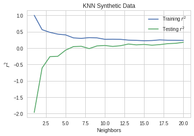
I originally had it set to a maximum of 10 neighbors, which made it appear that 9 was the peak, but expanding it shows that it was 15. It had a fairly low \(r^2\) score, even at its best. There appears to be more variance in the make_regression function than I had thought. When I ran it earlier the testing score never exceeded the training score and the best k was 12. The actual best score was the same, though.
print("Max r2: {:.2f}".format(max(test_score)))
Max r2: 0.47
The default for the make_regression function is to create 100 samples (which I mimicked by passing in 100 explicitly). By statistics standards this is a reasonable dataset (I believe 20 samples was the minimum for a long time) but it is very small by machine learning samples. Will it do better if it has a larger sample size?
plot_r_squared(samples=1000)
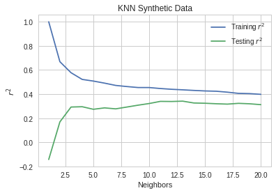
It didn't, but maybe because I didn't increase the number of neighbors.
plot_r_squared(neighbors=100, samples=1000)
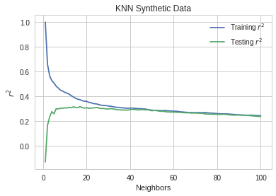
No, that didn't help, and after re-looking at the plot above I realized that it was getting worse at the end, so I shouldn't have expected that to help. So why does it do worse with more data?
train, test, models = plot_r_squared(samples=10000, neighbors=100)
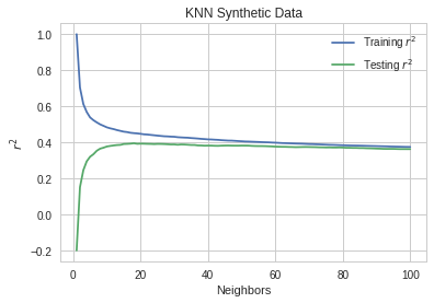
Having even more data seems to have improved the amount the testing score goes down with the number of neighbors. Maybe there's an ideal neighbors to data points ratio that I'm missing, and too many neighbors means you need more data.
@jit
def find_first(array, match):
    """find the index of the first match

    Expects a 1-dimensional array or list

    Args:
     array (numpy.array): thing to search
     match: thing to match

    Returns:
     int: index of the first match found (or None)
    """
    for index in range(len(array)):
        if array[index] == match:
            return index
    return
best = max(test)
print("Best Test r2: {:.2f}".format(best))
test = numpy.array(test)
index = find_first(test, best)
print("Best Neighbors: {0}".format(index + 1))
Best Test r2: 0.39
Best Neighbors: 18
Boston
This dataset was created to see if there was a correlation between polution and the price of houses in the Boston area.
Imports
import matplotlib.pyplot as pyplot
import seaborn
from sklearn.datasets import load_boston
from sklearn.model_selection import train_test_split
from sklearn.neighbors import KNeighborsRegressor
%matplotlib inline
seaborn.set_style("whitegrid")
The Data
boston = load_boston()
print("Boston data-shape: {0}".format(boston.data.shape))
Boston data-shape: (506, 13)
Boston House Prices dataset
Notes
Data Set Characteristics:
| Number of Instances: | |
|---|---|
| 506 | |
| Number of Attributes: | |
| 13 numeric/categorical predictive | |
| Median Value: | (attribute 14) is usually the target |
| Attribute Information (in order): | |
- CRIM per capita crime rate by town
- ZN proportion of residential land zoned for lots over 25,000 sq.ft.
- INDUS proportion of non-retail business acres per town
- CHAS Charles River dummy variable (= 1 if tract bounds river; 0 otherwise)
- NOX nitric oxides concentration (parts per 10 million)
- RM average number of rooms per dwelling
- AGE proportion of owner-occupied units built prior to 1940
- DIS weighted distances to five Boston employment centres
- RAD index of accessibility to radial highways
- TAX full-value property-tax rate per $10,000
- PTRATIO pupil-teacher ratio by town
- B 1000(Bk - 0.63)^2 where Bk is the proportion of blacks by town
- LSTAT % lower status of the population
- MEDV Median value of owner-occupied homes in $1000's
| Missing Attribute Values: | |
|---|---|
| None | |
| Creator: | Harrison, D. and Rubinfeld, D.L. |
This is a copy of UCI ML housing dataset. http://archive.ics.uci.edu/ml/datasets/Housing
This dataset was taken from the StatLib library which is maintained at Carnegie Mellon University.
The Boston house-price data of Harrison, D. and Rubinfeld, D.L. 'Hedonic prices and the demand for clean air', J. Environ. Economics & Management, vol.5, 81-102, 1978. Used in Belsley, Kuh & Welsch, 'Regression diagnostics ...', Wiley, 1980. N.B. Various transformations are used in the table on pages 244-261 of the latter.
The Boston house-price data has been used in many machine learning papers that address regression problems.
References
- Belsley, Kuh & Welsch, 'Regression diagnostics: Identifying Influential Data and Sources of Collinearity', Wiley, 1980. 244-261.
- Quinlan,R. (1993). Combining Instance-Based and Model-Based Learning. In Proceedings on the Tenth International Conference of Machine Learning, 236-243, University of Massachusetts, Amherst. Morgan Kaufmann.
- many more! (see http://archive.ics.uci.edu/ml/datasets/Housing)
print(boston.keys())
dict_keys(['target', 'feature_names', 'data', 'DESCR'])
This time there's no target-names because it is a regression problem instead of a classification problem.
X_train, X_test, y_train, y_test = train_test_split(boston.data, boston.target)
Model Performance
def get_r_squared(max_neighbors=10):
    train_score = []
    test_score = []
    models = []
    for neighbors in range(1, max_neighbors+1):
        model = KNeighborsRegressor(n_neighbors=neighbors)
        model.fit(X_train, y_train)
        train_score.append(model.score(X_train, y_train))
        test_score.append(model.score(X_test, y_test))
        models.append(model)
    return train_score, test_score, models
train_score, test_score, models = get_r_squared()
neighbors = range(1, 11)
pyplot.plot(neighbors, train_score, label="Training $r^2$")
pyplot.plot(neighbors, test_score, label="Testing $r^2$")
pyplot.xlabel("Neighbors")
pyplot.ylabel("$r^2$")
pyplot.title("KNN Boston Housing Prices")
pyplot.legend()
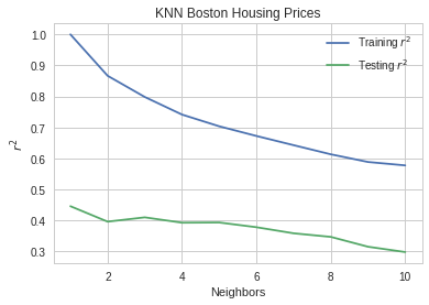
The testing score seems to peak at 2 neighbors and then go down from there.
print("Training r2 for 2 neigbors: {:.2f}".format(train_score[1]))
print("Testing r2 for 2 neighbors: {:.2f}".format(test_score[1]))
assert max(test_score) == test_score[1]
Training r2 for 2 neigbors: 0.84
Testing r2 for 2 neighbors: 0.63
In this case the K-Nearest Neighbors didn't seem to do as well with regression as it did with classification.