Visualizing Naive Bayes

Beginning

In the previous post I made a class-based version of the Naive Bayes Classifier for tweets. For this post I'm going to plot the model values. It turns out that we need to get at some values that the previous implementations hide so I'm going to re-calculate the likelihoods from scratch rather than alter the previous code.

Set Up

Imports

# python
from argparse import Namespace
from functools import partial
from pathlib import Path

import os
import pickle

# from pypi
from dotenv import load_dotenv
from matplotlib.patches import Ellipse

import holoviews
import hvplot.pandas
import matplotlib.pyplot as pyplot
import matplotlib.transforms as transforms
import numpy
import pandas
import seaborn

# this project
from neurotic.nlp.twitter.counter import WordCounter

# graeae
from graeae import EmbedHoloviews

The Dotenv

env_path = Path("posts/nlp/.env")
assert env_path.is_file()
load_dotenv(env_path)

Plotting

SLUG = "visualizing-naive-bayes"
Embed = partial(EmbedHoloviews,
                folder_path=f"files/posts/nlp/{SLUG}", create_folder=False)

plot_path = Path(os.environ["TWITTER_PLOT"])
assert plot_path.is_file()
with plot_path.open("rb") as reader:
    Plot = pickle.load(reader)
seaborn.set_style("whitegrid", rc={"axes.grid": False})
FIGURE_SIZE = (12, 10)

The Data

train_raw = pandas.read_feather(
    Path(os.environ["TWITTER_TRAINING_RAW"]).expanduser())

test_raw = pandas.read_feather(
    Path(os.environ["TWITTER_TEST_RAW"]).expanduser()
)

print(f"Training: {len(train_raw):,}")
print(f"Testing: {len(test_raw):,}")
Training: 8,000
Testing: 2,000

The Word Counter

This is a class to clean and tokenize the tweets and build up a Counter with the word counts.

counter = WordCounter(train_raw.tweet, train_raw.label)

Constants

Sentiment = Namespace(
    positive = 1,
    negative = 0,
)

Middle

Log Likelihoods

Calculating the Likelihoods

The first thing to plot are the log-likelihoods for positive and negative tweets. When I implemented the Naive Bayes Classifier I took advantage of the fact that we're making a binary classifier and took the odds ratio when making predictions, but for our plot we're going to need to undo the division and plot the numerator against the denominator.

\begin{align} log \frac{P(tweet|pos)}{P(tweet|neg)} &= log(P(tweet|pos)) - log(P(tweet|neg)) \\ positive = log(P(tweet|pos)) &= \sum_{i=0}^{n}{log P(W_i|pos)}\\ negative = log(P(tweet|neg)) &= \sum_{i=0}^{n}{log P(W_i|neg)}\\ \end{align}

So, let's get the log-likelihoods.

COUNTS = counter.counts

positive_loglikelihood = {}
negative_loglikelihood = {}
log_ratio = {}

all_positive_words = sum(
    (counts[(token, sentiment)] for token, sentiment in COUNTS
     if sentiment == Sentiment.positive))
all_negative_words = sum(
    (counts[(token, sentiment)] for token, sentiment in COUNTS
     if sentiment == Sentiment.negative))

vocabulary = {key[0] for key in COUNTS}
vocabulary_size = len(vocabulary)

for word in vocabulary:
    this_word_positive_count = COUNTS[(word, Sentiment.positive)]
    this_word_negative_count = COUNTS[(word, Sentiment.negative)]

    probability_word_is_positive = ((this_word_positive_count + 1)/
                                    (all_positive_words + vocabulary_size))
    probability_word_is_negative = ((this_word_negative_count + 1)/
                                    (all_negative_words + vocabulary_size))
    positive_loglikelihood[word] = numpy.log(probability_word_is_positive)
    negative_loglikelihood[word] = numpy.log(probability_word_is_negative)
    log_ratio[word] = positive_loglikelihood[word] - negative_loglikelihood[word]

So now we have our positive and negative log-likelihoods and I'll put them into a pandas DataFrame to make it easier to plot.

positive_document_likelihood = []
negative_document_likelihood = []
sentiment = []

for row in train_raw.itertuples():
    tokens = counter.process(row.tweet)

    positive_document_likelihood.append(sum(positive_loglikelihood.get(token, 0)
                                            for token in tokens))
    negative_document_likelihood.append(sum(negative_loglikelihood.get(token, 0)
                                            for token in tokens))
    sentiment.append(row.label)

features = pandas.DataFrame.from_dict(
    dict(
        positive = positive_document_likelihood,
        negative = negative_document_likelihood,
        sentiment=sentiment,
    )
)

print(features.head())
     positive   negative  sentiment
0  -26.305672 -33.940649          1
1  -30.909803 -37.634516          1
2  -42.936400 -33.403567          0
3  -15.983546 -25.501140          1
4 -107.899933 -99.191875          0

Plotting the Likelihoods

plot = features.hvplot.scatter(x="positive", y="negative", by="sentiment",
                               color=Plot.color_cycle, fill_alpha=0).opts(
                                   title="Positive vs Negative",
                                   width=Plot.width,
                                   height=Plot.height,
                                   fontscale=Plot.font_scale,
                               )

outcome = Embed(plot=plot, file_name="positive_vs_negative_sentiment")()
print(outcome)

Figure Missing

It looks like the log likelihoods for the negatives are linearly separable.

Confidence Ellipses

Now we're going to plot a Confidence Region, which is a generalization of a confidence interval to higher dimensions. In this case we're going to create confidence ellipses. I'm not really sure about the details of the math to get them, but matplotlib has a page with a function to create a matplotlib plot for a confidence ellipse that I'm going to adapt.

The Ellipse Function

This is taken almost verbatim from matplotlib's page.

def confidence_ellipse(x, y, ax, n_std=3.0, facecolor='none', **kwargs):
    """
    Create a plot of the covariance confidence ellipse of `x` and `y`

    Parameters
    ----------
    x, y : array_like, shape (n, )
       Input data.

    ax : matplotlib.axes.Axes
       The axes object to draw the ellipse into.

    n_std : float
       The number of standard deviations to determine the ellipse's radiuses.

    Returns
    -------
    matplotlib.patches.Ellipse

    Other parameters
    ----------------
    kwargs : `~matplotlib.patches.Patch` properties
    """
    if x.size != y.size:
        raise ValueError("x and y must be the same size")

    cov = numpy.cov(x, y)
    pearson = cov[0, 1]/numpy.sqrt(cov[0, 0] * cov[1, 1])
    # Using a special case to obtain the eigenvalues of this
    # two-dimensionl dataset.
    ell_radius_x = numpy.sqrt(1 + pearson)
    ell_radius_y = numpy.sqrt(1 - pearson)
    ellipse = Ellipse((0, 0),
                      width=ell_radius_x * 2,
                      height=ell_radius_y * 2,
                      facecolor=facecolor,
                      **kwargs
                      )

    # Calculating the stdandard deviation of x from
    # the squareroot of the variance and multiplying
    # with the given number of standard deviations.
    scale_x = numpy.sqrt(cov[0, 0]) * n_std
    mean_x = numpy.mean(x)

    # calculating the stdandard deviation of y ...
    scale_y = numpy.sqrt(cov[1, 1]) * n_std
    mean_y = numpy.mean(y)

    transf = transforms.Affine2D() \
        .rotate_deg(45) \
        .scale(scale_x, scale_y) \
        .translate(mean_x, mean_y)

    ellipse.set_transform(transf + ax.transData)
    return ax.add_patch(ellipse)
figure, axis = pyplot.subplots(figsize = (12, 12))

positives = features[features.sentiment==Sentiment.positive]
negatives = features[features.sentiment==Sentiment.negative]

confidence_ellipse(positives.positive, positives.negative, axis, n_std=2,
                   label=r'$2\sigma$', edgecolor=Plot.red)
confidence_ellipse(negatives.positive, negatives.negative, axis, n_std=2, edgecolor=Plot.blue)

confidence_ellipse(positives.positive, positives.negative, axis, n_std=3,
                   label=r'$3\sigma$', edgecolor=Plot.red)
confidence_ellipse(negatives.positive, negatives.negative, axis, n_std=3, edgecolor=Plot.blue)

SIZE = 0.5
_ = positives.plot.scatter(x="positive", y="negative", s=SIZE, ax=axis, facecolors="none",
                           color=Plot.blue, label="positive")
negatives.plot.scatter(x="positive", y="negative", s=SIZE, ax=axis,
                       label="negative", color=Plot.red)

LIMITS = (-200, 100)
axis.set_xlim(LIMITS)
axis.set_ylim(LIMITS)
axis.legend()
axis.set_title("Confidence Ellipses")

figure.savefig("ellipses.png")

ellipses.png

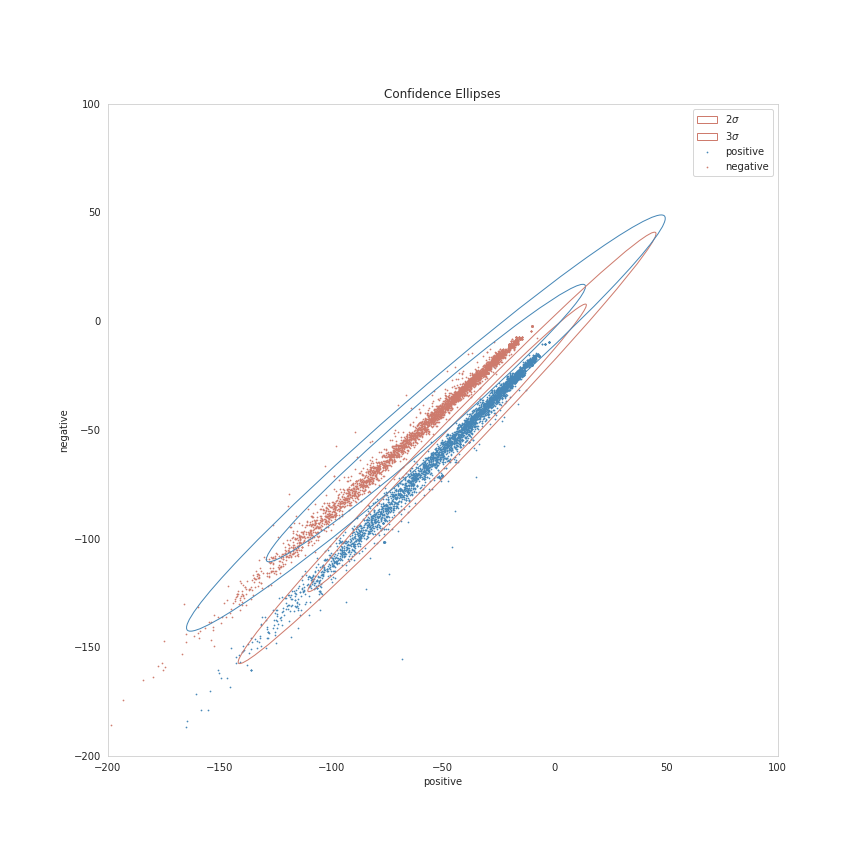
It's a bit squashed looking, since the results are so tight, but you can sort of see that the distributions are "left-skewed", with the points that fall outside of the \(3 \sigma\) range being the cases where the "positive" and "negative" values are both negative.

End

Class-Based Naive Bayes Tweet Sentiment Classifier

Beginning

I previously implemented a Naive Bayes Classifier for Tweets as separate functions, and while that is useful for learningi I want to re-use it so I'm going to re-implement it as a class-based system.

The Naive Bayes Classifier

Imports

# python
from argparse import Namespace
from collections import Counter
from typing import Iterable

# pypi
import attr
import numpy

# my stuff
from neurotic.nlp.twitter.counter import WordCounter

The Sentiment Constants

Sentiment = Namespace(
    negative = 0,
    positive = 1,
)

The Declaration

@attr.s(auto_attribs=True)
class NaiveBayes:
    """Naive Bayes Sentiment Classifier for Tweets

    Args:
     tweets: the training tweets
     labels: the sentiment labels for the training tweets
    """
    tweets: Iterable
    labels: Iterable
    _counter: WordCounter = None
    _vocabulary: set = None
    _logprior: float = None
    _loglikelihood: dict = None

The Counter

@property
def counter(self) -> WordCounter:
    """The word processor/counter"""
    if self._counter is None:
        self._counter = WordCounter(self.tweets, self.labels)
    return self._counter

The Vocabulary

@property
def vocabulary(self) -> set:
    """The unique tokens in the tweets"""
    if self._vocabulary is None:
        self._vocabulary = {key[0] for key in self.counter.counts}
    return self._vocabulary

The logprior

@property
def logprior(self) -> float:
    """the log-odds of the priors"""
    if self._logprior is None:
        positive_documents = numpy.sum(self.labels)
        negative_documents = len(self.labels) - positive_documents
        self._logprior = numpy.log(positive_documents) - numpy.log(negative_documents)
    return self._logprior

The loglikelihood

@property
def loglikelihood(self) -> dict:
    """The log-likelihoods for words"""
    if self._loglikelihood is None:
        self._loglikelihood = {}
        counts = self.counter.counts        

        all_positive_words = sum(
            (counts[(token, sentiment)] for token, sentiment in counts
             if sentiment == Sentiment.positive))
        all_negative_words = sum(
            (counts[(token, sentiment)] for token, sentiment in counts
             if sentiment == Sentiment.negative))
        vocabulary_size = len(self.vocabulary)

        for word in self.vocabulary:
            this_word_positive_count = counts[(word, Sentiment.positive)]
            this_word_negative_count = counts[(word, Sentiment.negative)]

            probability_word_is_positive = ((this_word_positive_count + 1)/
                                         (all_positive_words + vocabulary_size))
            probability_word_is_negative = ((this_word_negative_count + 1)/
                                         (all_negative_words + vocabulary_size))

            self._loglikelihood[word] = (numpy.log(probability_word_is_positive) -
                                         numpy.log(probability_word_is_negative))
    return self._loglikelihood

Predict Probability

def predict_ratio(self, tweet: str) -> float:
    """predict the odds-ratio positive/negative

    Args:
     tweet: the tweet to predict

    Returns:
     log-odds-ratio for tweet (positive/negative)
    """
    tokens = self.counter.process(tweet)
    return self.logprior + sum(self.loglikelihood.get(token, 0) for token in tokens)

Predict Sentiment

def predict_sentiment(self, tweet: str) -> int:
    """Predict whether the tweet's sentiment is positive or negative

    Args:
     tweet: the 'document' to analyze

    Returns:
     the sentiment (0=negative, 1=positive)
    """
    return self.predict_ratio(tweet) > 0

Check Rep

def check_rep(self) -> None:
    """Does some basic checks of the input arguments"""
    assert len(self.tweets) == len(self.labels)
    return

Testing

Imports

"""NaiveBayes Tweet Sentiment Classifier feature tests."""

# python
from collections import Counter

import math

# pypi
from expects import (
    be,
    be_empty,
    be_true,
    equal,
    expect,
)

from pytest_bdd import (
    given,
    scenarios,
    then,
    when,
)

import pytest_bdd

# this test repo
from fixtures import katamari

# software under test
from neurotic.nlp.twitter.counter import WordCounter
from neurotic.nlp.twitter.naive_bayes import NaiveBayes

Test Setup

scenarios("../../features/twitter/naive_bayes.feature")

Can you construct it?

Feature: NaiveBayes Tweet Sentiment Classifier

Scenario: The user builds the classifier
  Given a Naive Bayes definition
  When the user builds the classifier
  Then it has the expected attributes
# Scenario: The user builds the classifier


@given('a Naive Bayes definition')
def a_naive_bayes_definition(katamari):
    katamari.definition = NaiveBayes
    return


@when('the user builds the classifier')
def the_user_builds_the_classifier(katamari):
    katamari.labels = [0, 1, 1]
    katamari.tweets = "alfa bravo charley".split()
    katamari.classifier = katamari.definition(tweets=katamari.tweets,
                                              labels=katamari.labels)
    return


@then('it has the expected attributes')
def it_has_the_expected_attributes(katamari):
    expect(katamari.classifier.tweets).to(be(katamari.tweets))
    expect(katamari.classifier.labels).to(be(katamari.labels))
    katamari.classifier.check_rep()
    return

Does it build the counter?

Scenario: The user checks the counter
  Given a Naive Bayes classifier
  When the user checks the counter
  Then it is the expected counter
# Scenario: The user checks the counter

@given("a Naive Bayes classifier")
def build_naive_classifier(katamari):
    katamari.classifier = NaiveBayes(tweets=[], labels=[])
    return


@when("the user checks the counter")
def check_counter(katamari, mocker):
    katamari.counter = mocker.MagicMock(spec=WordCounter)
    katamari.counter_definition = mocker.MagicMock()
    katamari.counter_definition.return_value = katamari.counter
    mocker.patch("neurotic.nlp.twitter.naive_bayes.WordCounter", katamari.counter_definition)
    katamari.actual_counter = katamari.classifier.counter
    return


@then("it is the expected counter")
def expect_counter(katamari):
    expect(katamari.actual_counter).to(be(katamari.counter))
    return

Does it build the logprior?

Scenario: The user checks the log-prior
 Given a valid Naive Bayes Classifier
 When the user checks the log-odds prior
 Then it is close enough
# Scenario: The user checks the log-prior

@given("a valid Naive Bayes Classifier")
def setup_classifier(katamari):
    katamari.tweets = ["a blowfish", "b closing", "c that", "d plane"]
    katamari.labels = [1, 1, 0, 1]
    katamari.counts = Counter({
        ("appl", 0): 5,
        ("b", 1): 2,
        ("c", 1): 4,

    })
    katamari.classifier = NaiveBayes(tweets=katamari.tweets,
                                     labels = katamari.labels)
    katamari.classifier.counter._counts = katamari.counts
    return


@when("the user checks the log-odds prior")
def get_log_odds_prior(katamari):
    katamari.expected = math.log(3) - math.log(1)
    katamari.actual = katamari.classifier.logprior
    return


@then("it is close enough")
def expect_close_enough(katamari):
    expect(math.isclose(katamari.actual, katamari.expected)).to(be_true)
    return

Does it build the vocabulary?

Scenario: The user checks the vocabulary
  Given a valid Naive Bayes Classifier
  When the user checks the vocabulary
  Then all the words are there
# Scenario: The user checks the vocabulary
#  Given a valid Naive Bayes Classifier


@when("the user checks the vocabulary")
def check_vocabulary(katamari):
  katamari.actual = katamari.classifier.vocabulary
  katamari.expected = {"appl", "b", "c"}
  return


@then("all the words are there")
def compare_words(katamari):
  expect(katamari.actual ^ katamari.expected).to(be_empty)
  return

Does it build the log-likelihood?

Scenario: The user gets the log-likelihood dictionary
  Given a valid Naive Bayes Classifier
  When the user checks the loglikelihoods
  Then they are close enough
# Scenario: The user gets the log-likelihood dictionary
#  Given a valid Naive Bayes Classifier


@when("the user checks the loglikelihoods")
def check_log_likelihoods(katamari):
    katamari.expected = dict(
        appl=math.log(1/9) - math.log(6/8),
        b=math.log(3/9) - math.log(1/8),
        c=math.log(5/9) - math.log(1/8)
    )
    katamari.actual = katamari.classifier.loglikelihood
    return


@then("they are close enough")
def expect_close_values(katamari):
    for word in katamari.classifier.loglikelihood:
        expect(math.isclose(katamari.expected[word],
                            katamari.actual[word])).to(be_true)
    return

Does it predict probabilities?

Scenario: User predicts tweet positive probability
  Given a valid Naive Bayes Classifier
  When the user makes a tweet prediction
  Then it is the expected probability
# Scenario: User predicts tweet positive probability
#   Given a valid Naive Bayes Classifier


@when("the user makes a tweet prediction")
def check_prediction(katamari):
    katamari.expected = (katamari.classifier.logprior
                         + katamari.classifier.loglikelihood["c"]
                         + katamari.classifier.loglikelihood["b"])
    katamari.actual = katamari.classifier.predict_ratio(
        "c you later b"
    )
    return


@then("it is the expected probability")
def expect_probability(katamari):
    expect(math.isclose(katamari.actual, katamari.expected)).to(be_true)
    return

Does it predict the sentiment?

Scenario: The user predicts tweet sentiment
  Given a valid Naive Bayes Classifier
  When the user predicts the sentiment of tweets
  Then the sentiments are the expected ones
# Scenario: The user predicts tweet sentiment
#   Given a valid Naive Bayes Classifier


@when("the user predicts the sentiment of tweets")
def check_predict_sentiment(katamari):
    katamari.actual_1 = katamari.classifier.predict_sentiment("c you later b")
    katamari.expected_1 = 1

    katamari.actual_2 = katamari.classifier.predict_sentiment("apple banana tart")
    katamari.expected_2 = 0
    return


@then("the sentiments are the expected ones")
def expect_sentiments(katamari):
    expect(katamari.actual_1).to(equal(katamari.expected_1))
    expect(katamari.actual_2).to(equal(katamari.expected_2))
    return

End

Now that we have the class-based version let's do a little visualization of the model.

Implementing a Naive Bayes Twitter Sentiment Classifier

Beginning

In the previous post I went through some of the background of how Naive Bayes works. In this post I'll implement a Naive Bayes Classifier to classify tweets by whether they are positive in sentiment or negative. The Naive Bayes model uses Bayes' rule to make its predictions and it's called "naive" because it makes the assumption that words in the document are independent (in the probability event sense) which allows us to use the multiplication rule to calculate our probabilities. It also uses the \(\textit{Bag of Words}\) assumption that word ordering isn't important.

Set Up

This first bit imports the needed dependencies followed by setting up the data and some helpers.

Imports

# python
from collections import Counter, defaultdict
from functools import partial
from pathlib import Path

import os
import pickle

# pypi
from dotenv import load_dotenv
from tabulate import tabulate

import numpy
import pandas

# my stuff
from neurotic.nlp.twitter.counter import WordCounter

Tabulate

This sets up tabulate to make it a little simpler to display pandas DataFrames in org.

TABLE = partial(tabulate, tablefmt="orgtbl", headers="keys", showindex=False)

The Dotenv

I put the path to the data files in a .env file so this loads it into the environment.

env_path = Path("posts/nlp/.env")
assert env_path.is_file()
load_dotenv(env_path)

Load the Twitter Data

I split the data previously for the Logistic Regression twitter sentiment classifier so I'll load it here and skip building the sets.

train_raw = pandas.read_feather(
    Path(os.environ["TWITTER_TRAINING_RAW"]).expanduser())

test_raw = pandas.read_feather(
    Path(os.environ["TWITTER_TEST_RAW"]).expanduser()
)

print(f"Training: {len(train_raw):,}")
print(f"Testing: {len(test_raw):,}")
Training: 8,000
Testing: 2,000

I'll also re-use the WordCounter from the Logistic Regression. Despite the name it also does tokenizing and cleaning.

counter = WordCounter(train_raw.tweet, train_raw.label)

Constants

This was an object I created to store a few constant values.

with open(os.environ["TWITTER_SENTIMENT"], "rb") as reader:
    Sentiment = pickle.load(reader)
print(Sentiment)
Namespace(decode={1: 'positive', 0: 'negative'}, encode={'positive': 1, 'negative': 0}, negative=0, positive=1)

Middle

Implementing the Model

In an earlier post I wrote up a little of the background behind what we're doing and now I'm going to translate the math in that post into code.

Implementing The Training Function

The first part of the problem - training the model by building up the probabilities.

def train_naive_bayes(counts: Counter,
                      train_x: pandas.Series,
                      train_y: pandas.Series) -> tuple:
    """
    Args:
       counts: Counter from (word, label) to how often the word appears
       train_x: a list of tweets
       train_y: a list of labels correponding to the tweets (0,1)

    Returns:
       logprior: the log odds ratio
       loglikelihood: log likelihood dictionary for the Naive bayes equation
    """
    loglikelihood = defaultdict(lambda: 0)
    logprior = 0

    vocabulary = set([pair[0] for pair in counts])
    V = len(vocabulary)

    # number of positive and negative words in the training set
    N_pos = sum((counts[(token, sentiment)] for token, sentiment in counts
                 if sentiment == Sentiment.positive))
    N_neg = sum((counts[(token, sentiment)] for token, sentiment in counts
                 if sentiment == Sentiment.negative))

    D = len(train_x)

    # D_pos is number of positive documents
    D_pos = train_y.sum()

    # D_neg is the number of negative documents
    D_neg = D - D_pos

    # the log odds ratio
    logprior = numpy.log(D_pos) - numpy.log(D_neg)

    for word in vocabulary:
        freq_pos = counts[(word, Sentiment.positive)]
        freq_neg = counts[(word, Sentiment.negative)]

        # the probability that the word is positive, and negative
        p_w_pos = (freq_pos + 1)/(N_pos + V)
        p_w_neg = (freq_neg + 1)/(N_neg + V)

        loglikelihood[word] = numpy.log(p_w_pos) - numpy.log(p_w_neg)
    return logprior, loglikelihood

Now we can see what we get when we train our model.

logprior, loglikelihood = train_naive_bayes(counter.counts, train_raw.tweet, train_raw.label)
print(f"Log Prior: {logprior}")
print(f"Words in Log Likelihood: {len(loglikelihood):,}")
Log Prior: -0.006500022885560952
Words in Log Likelihood: 9,172
print(f"Positive Tweets: {len(train_raw[train_raw.label==Sentiment.positive]):,}")
print(f"Negative Tweets: {len(train_raw[train_raw.label==Sentiment.negative]):,}")
Positive Tweets: 3,987
Negative Tweets: 4,013

We get a negative value for the logprior because we have more negative tweets than positive tweets in the training set and the negative count is the second term when we calculate the difference for the logprior. If we evened it out it would drop to 0.

all_raw = pandas.concat([train_raw, test_raw])
check = pandas.concat([
    all_raw[all_raw.label==1].iloc[:4000], all_raw[all_raw.label==0].iloc[:4000]])
logprior, loglikelihood = train_naive_bayes(counter.counts, check.tweet, check.label)
print(f"Log Prior: {logprior}")
print(f"Log Likelihood: {len(loglikelihood)}")
Log Prior: 0.0
Log Likelihood: 9172

Making Predictions

Now that we have the model we can use it to make some predictions.

\[ p = logprior + \sum_i^N (loglikelihood_i) \]

def naive_bayes_predict(tweet: str, logprior: float, loglikelihood: dict) -> float:
    """
    Args:
       tweet: a tweet to classify
       logprior: the log odds ratio of prior probabilities
       loglikelihood: a dictionary of words mapped to their log likelihood ratios

    Returns:
       p: sum of the log-odds ratio for the tweet
    """
    # process the tweet to get a list of words
    words = counter.process(tweet)
    return logprior + sum(loglikelihood[word] for word in words)

Now test it with a tweet.

my_tweet = 'She smiled.'
p = naive_bayes_predict(my_tweet, logprior, loglikelihood)
print(f'The positive to negative ratio is {p:0.2f}.')
The positive to negative ratio is 1.44.

Since the ratio is greater than 0, we're predicting that the tweet has a positive sentiment.

Test The Model

Now we'll calculate the accuracy of the model against the test set.

def test_naive_bayes(test_x: pandas.Series, test_y: pandas.Series,
                     logprior: float, loglikelihood: dict) -> float:
    """
    Args:
       test_x: tweets to classify
       test_y: labels for test_x
       logprior: the logprior for the training set
       loglikelihood: a dictionary with the loglikelihoods for each word

    Returns:
       accuracy: (# of tweets classified correctly)/(total # of tweets)
    """
    accuracy = 0

    y_hats = numpy.array([int(naive_bayes_predict(tweet, logprior, loglikelihood) > 0)
              for tweet in test_x])

    # error is the average of the absolute values of the differences between y_hats and test_y
    # error = number wrong/number of tweets
    error = numpy.abs(y_hats - test_y).mean()

    # Accuracy is 1 minus the error
    accuracy = 1 - error
    return accuracy
print("Naive Bayes accuracy = %0.4f" %
      (test_naive_bayes(test_raw.tweet, test_raw.label, logprior, loglikelihood)))
Naive Bayes accuracy = 0.9955

Which looks good, but it might actually be overfitting - it looks too good. Now here's some example tweets to check.

for tweet in ['I am happy', 'I am bad', 'this movie should have been great.',
              'great', 'great great', 'great great great', 'great great great great']:
    p = naive_bayes_predict(tweet, logprior, loglikelihood)
    print(f'{tweet} -> {p:.2f}')
I am happy -> 1.89
I am bad -> -1.63
this movie should have been great. -> 2.05
great -> 2.06
great great -> 4.13
great great great -> 6.19
great great great great -> 8.25

It looks like the word "great" throws off the third sentence which hints at being negative. What if we pass in a neutral (nonsensical) tweet?

my_tweet = "the answer is nicht in the umwelt"
print(naive_bayes_predict(my_tweet, logprior, loglikelihood))
-0.41441957689474407

I don't know which of those words triggered the negative value…

for word in "the answer is nicht in the umwelt".split():
    print(f"{word}:\t{naive_bayes_predict(word, logprior, loglikelihood):0.2f}")
the:    0.00
answer: -0.41
is:     0.00
nicht:  0.00
in:     0.00
the:    0.00
umwelt: 0.00

It only got one word, answer and that's negative for some reason. Go figure.

Filtering Words

This is sort of an aside, but one way to quickly filter tweets based on how positive or negative they are is to use the ratio of positive to negative counts and setting a threshold that has to be met to be included in the output.

\[ ratio = \frac{\text{pos_words} + 1}{\text{neg_words} + 1} \]

Words Positive word count Negative Word Count
glad 41 2
arriv 57 4
:( 1 3663
:-( 0 378

Get The Ratio

As an intermediate step we'll create a function named get_ratio that looks up a word and calculates the positive to negative ratio.

def get_ratio(freqs: Counter, word: str) -> dict:
    """
    Args:
       freqs: Counter with (word, sentiment) : count
       word: string to lookup

    Returns: 
     dictionary with keys 'positive', 'negative', and 'ratio'.
       Example: {'positive': 10, 'negative': 20, 'ratio': 0.5}
    """
    pos_neg_ratio = dict(
        positive = freqs[(word, Sentiment.positive)],
        negative = freqs[(word, Sentiment.negative)],
    )

    # calculate the ratio of positive to negative counts for the word
    pos_neg_ratio['ratio'] = (pos_neg_ratio["positive"] + 1)/(
        pos_neg_ratio["negative"] + 1)
    return pos_neg_ratio
print(get_ratio(counter.counts, 'happi'))
{'positive': 160, 'negative': 23, 'ratio': 6.708333333333333}

Get Words By Threshold

Now we'll create the filter function. To make it simpler we'll assume that if we're filtering on the positive label then the ratio for a word to be included has to be equal to or greater than the given threshold while if the label is negative then a word has to be less than or equal to the threshold. Doing this means we're filtering to get words that are further toward the extremes of positive or negative (further from 0).

An example key-value pair would have this structure:

{'happi':
     {'positive': 10, 'negative': 20, 'ratio': 0.5}
 }
def get_words_by_threshold(freqs: Counter, label: int, threshold: float) -> dict:
    """
    Args:
       freqs: Counter of (word, sentiment): word count
       label: 1 for positive, 0 for negative
       threshold: ratio that will be used as the cutoff for including a word in the returned dictionary

    Returns:
       words: dictionary containing the word and information on its positive count, negative count, and ratio of positive to negative counts.
       example of a key value pair:
       {'happi':
           {'positive': 10, 'negative': 20, 'ratio': 0.5}
       }
    """
    words = {}

    for word, _ in freqs:
        pos_neg_ratio = get_ratio(freqs, word)

        if ((label == Sentiment.positive and pos_neg_ratio["ratio"] >= threshold) or
            (label == Sentiment.negative and pos_neg_ratio["ratio"] <= threshold)):
            words[word] = pos_neg_ratio

    return words

Here's an example where we'll filter on negative sentiment so all the tweets should be negative and have a positive to negative ration less that the threshold.

passed = get_words_by_threshold(counter.counts, label=Sentiment.negative, threshold=0.05)
count = 1
for word, info in passed.items():
    print(f"{count}\tword: {word}\t{info}")
    count += 1
1       word: :(        {'positive': 1, 'negative': 3705, 'ratio': 0.0005396654074473826}
2       word: :-(       {'positive': 0, 'negative': 407, 'ratio': 0.0024509803921568627}
3       word: ♛ {'positive': 0, 'negative': 162, 'ratio': 0.006134969325153374}
4       word: 》 {'positive': 0, 'negative': 162, 'ratio': 0.006134969325153374}
5       word: beli̇ev   {'positive': 0, 'negative': 27, 'ratio': 0.03571428571428571}
6       word: wi̇ll     {'positive': 0, 'negative': 27, 'ratio': 0.03571428571428571}
7       word: justi̇n   {'positive': 0, 'negative': 27, 'ratio': 0.03571428571428571}
8       word: see       {'positive': 0, 'negative': 27, 'ratio': 0.03571428571428571}
9       word: me        {'positive': 0, 'negative': 27, 'ratio': 0.03571428571428571}
10      word: sad       {'positive': 3, 'negative': 100, 'ratio': 0.039603960396039604}
11      word: >:(    {'positive': 0, 'negative': 36, 'ratio': 0.02702702702702703}

So our threshold gives us the eleven most negative words.

Now, what about filtering on the most positive words?

passed = get_words_by_threshold(counter.counts, label=Sentiment.positive, threshold=10)
count = 1
for word, info in passed.items():
    print(f"{count}\tword: {word}\t{info}")
    count += 1
1       word: :)        {'positive': 2967, 'negative': 1, 'ratio': 1484.0}
2       word: :-)       {'positive': 547, 'negative': 0, 'ratio': 548.0}
3       word: :D        {'positive': 537, 'negative': 0, 'ratio': 538.0}
4       word: :p        {'positive': 113, 'negative': 0, 'ratio': 114.0}
5       word: fback     {'positive': 22, 'negative': 0, 'ratio': 23.0}
6       word: blog      {'positive': 29, 'negative': 2, 'ratio': 10.0}
7       word: followfriday      {'positive': 19, 'negative': 0, 'ratio': 20.0}
8       word: recent    {'positive': 9, 'negative': 0, 'ratio': 10.0}
9       word: stat      {'positive': 52, 'negative': 0, 'ratio': 53.0}
10      word: arriv     {'positive': 57, 'negative': 4, 'ratio': 11.6}
11      word: thx       {'positive': 11, 'negative': 0, 'ratio': 12.0}
12      word: here'     {'positive': 19, 'negative': 0, 'ratio': 20.0}
13      word: influenc  {'positive': 16, 'negative': 0, 'ratio': 17.0}
14      word: bam       {'positive': 34, 'negative': 0, 'ratio': 35.0}
15      word: warsaw    {'positive': 34, 'negative': 0, 'ratio': 35.0}
16      word: welcom    {'positive': 58, 'negative': 4, 'ratio': 11.8}
17      word: vid       {'positive': 9, 'negative': 0, 'ratio': 10.0}
18      word: ceo       {'positive': 9, 'negative': 0, 'ratio': 10.0}
19      word: 1month    {'positive': 9, 'negative': 0, 'ratio': 10.0}
20      word: flipkartfashionfriday     {'positive': 14, 'negative': 0, 'ratio': 15.0}
21      word: inde      {'positive': 10, 'negative': 0, 'ratio': 11.0}
22      word: glad      {'positive': 35, 'negative': 2, 'ratio': 12.0}
23      word: braindot  {'positive': 9, 'negative': 0, 'ratio': 10.0}
24      word: ;)        {'positive': 21, 'negative': 0, 'ratio': 22.0}
25      word: goodnight {'positive': 19, 'negative': 1, 'ratio': 10.0}
26      word: youth     {'positive': 10, 'negative': 0, 'ratio': 11.0}
27      word: shout     {'positive': 9, 'negative': 0, 'ratio': 10.0}
28      word: fantast   {'positive': 10, 'negative': 0, 'ratio': 11.0}

The first four make sense, but after that maybe not so much. "fback"?

Error Analysis

Now let's look at some tweets that we got wrong. We're going to use numpy.sign which reduces numbers to -1, 0, or 1.

print('Truth Predicted Tweet')
for row in test_raw.itertuples():
    y_hat = naive_bayes_predict(row.tweet, logprior, loglikelihood)
    if row.label != (numpy.sign(y_hat) > 0):
        print(
            f"{row.label}\t{numpy.sign(y_hat) > 0:d}\t"
            f"{' '.join(counter.process(row.tweet)).encode('ascii', 'ignore')}")
Truth Predicted Tweet
0       1       b'whatev stil l young >:-('
1       0       b'look fun kik va 642 kik kikgirl french model orgasm hannib phonesex :)'
0       1       b'great news thank let us know :( hope good weekend'
0       1       b"amb pleas harry' jean :) ): ): ):"
0       1       b'srsli fuck u unfollow hope ur futur child unpar u >:-('
1       0       b'ate last cooki shir 0 >:d'
1       0       b'snapchat jennyjean 22 snapchat kikmeboy model french kikchat sabadodeganarseguidor sexysasunday :)'
1       0       b'add kik ughtm 545 kik kikmeguy kissm nude likeforfollow musicbiz sexysasunday :)'
0       1       b'sr financi analyst expedia inc bellevu wa financ expediajob job job hire'

For some reason it misses the >:-( emoji and the :) - maybe they didn't occur in the training set. I think these woud be hard for a human to get too, unless you were well versed in tweets and emojis and maybe even then it would be hard…

Predict Your Own Tweet

Let's try a random tweet not in the given training or test sets.

my_tweet = 'my balls itch'

p = naive_bayes_predict(my_tweet, logprior, loglikelihood)
print(f"{my_tweet} is a positive tweet: {numpy.sign(p) > 0}")
my balls itch is a positive tweet: True

Hmmm. Maybe…

End

I want to do more work with the Naive Bayes Classifier but this post is getting too long so I'm going to move on to other posts, the next being a class-based implementation of the model.

Using Naive Bayes to Classify Tweets by Sentiment

Table of Contents

Beginning

In a previous post I implemented a Logistic Regression model to classify twitter tweets as having a positive or negative sentiment. This time I'll be using the same data set (from NLTK) but implementing it with a Naive Bayes model. This post will look at some of the math behind it and the next one will translate the math into code.

Middle

Bayesian Inference

What we want is to take a document (D) - which is a tweet in this case - and guess its classification \(\hat{c}\). We do this by calculating the probability for both of our classifications (positive and negative) using Bayes' Rule and then choosing the classification with the higher probability.

\begin{align} \hat{c} &= \underset{c \in C}{\mathrm{argmax}} P(c|d)\\ &= \underset{c \in C}{\mathrm{argmax}} P(D|c)P(c)\\ \end{align}

So our guess as to what class the document belongs to is the classification with the highest probability given the document - and "the probability of the classification given the document", when translated using Bayes' Rule, becomes the probability of the document given the classification (the likelihood of the document) times the prior probability of any document belonging to the class. But then you might wonder - if there's only one of each document then won't the probability always be \(\frac{1}{c}\)? It would, so we use the words within the document to calculate the probability for the document. How? Well, I mentioned earlier that we make two assumptions - that the documents can be represented as a bag of words and that they are independent. The independent assumption allows us to figure out the total probability using the Multiplication Rule:

\[ P(A \cap B) = P(A)P(B) \]

The probability of A and B is the product of their probabilities. In this case we are calculating the probability of the document as the product of the conditional probabilities of the words given the class:

\[ P(D|c) = \prod_{i=1}^{n}P(w_i | c) \]

Where the n refers to the number of words in the document. Given this we could re-write the previous equation like this.

\begin{align} \hat{c} &= \underset{c \in C}{\textrm{argmax}} P(c) \prod_{i}^{n} P(w_i | c)\\ \end{align}

But it turns out this form isn't really ideal. Among other things you're multiplying values that range from 0 to 1, with most values being less than 1, so the more classes you have, the smaller this number will get and you could end up with really small numbers leading to underflow. So we're going to do a log transform of the equation which will also simplify the computation a little (although nowadays I don't know that that's so much of a consideration).

\[ \hat{c} = \underset{c \in C}{\textrm{argmax}} \log{P(c)} + \sum_{i=1}^n \log{P(w_i|c)} \]

This is what we'll use to classify tweets after training the model by building up the probabilities.

Ratios

While I wrote out the general case where you take the class with the highest probability, in this case we only have two classes, positive and negative so we can take advantage of this and make our classification using the ratio of the conditional probabilities for each class (the log odds ratio). We're going to use the ratio of positive to negative.

\[ \log{\frac{P(positive|D)}{P(negative | D)}} = \log{\frac{P(positive)}{P(negative)}} + \sum_{i=1}^n \log{\frac{P(w_i|positive)}{P(w_i|negative)}} \]

Since positive is the numerator, and the log of values less than one are negative, this ratio will be positive when the review is likely positive and negative otherwise, so we can use the sign of this ratio to classify tweets.

Priors and Log Priors

Now we can start picking apart our ratio. The prior probabilities are just the fraction of our training set that matches a variable. So the prior probabilities of the document classifications can be described like this:

\begin{align} P(D_{positive}) &= \frac{\textit{number of positive tweets}}{\textit{total number of tweets}}\\ &= \frac{D_{pos}}{D}\\ \end{align} \begin{align} P(D_{negative}) &= \frac{\textit{number of negative tweets}}{\textit{total number of tweets}}\\ &= \frac{D_{neg}}{D}\\ \end{align}

But as I noted above we are going to use the ratio of the prior probabilities \(\frac{P(D_{pos})}{P(D_{neg})}\) and if you look at them, they have the same denominator (D) so taking the ratio of the probabilities means the denominator cancels out and we end up with the ratio of the positive to negative documents.

\begin{align} \frac{P(D_{pos})}{P(D_{neg})} &= \frac{\frac{D_{pos}}{D}}{\frac{D_{neg}}{D}}\\ &= \frac{\left( \frac{D_{pos}}{\cancel{D}}\right) \left(\frac{\cancel{D}}{D_{neg}}\right) }{ \cancel{\left(\frac{D_{neg}}{D}\right)} \cancel{\left(\frac{D}{D_{neg}}\right)} }\\ &= \frac{D_{pos}}{D_{neg}}\\ \end{align}

And as I noted above, we'll be using a log transform so our ratio (which will be called logprior) needs to be transformed as well.

\begin{align} \text{logprior} &= log \left( \frac{P(D_{pos})}{P(D_{neg})} \right) \\ &= log \left( \frac{D_{pos}}{D_{neg}} \right)\\ \end{align}

Note that \(log(\frac{A}{B})\) is the same as \(log(A) - log(B)\). So the logprior can also be calculated as the difference between two logs:

\begin{align} \text{logprior} &= \log (P(D_{pos})) - \log (P(D_{neg})) \\ &= \log (D_{pos}) - \log (D_{neg})\\ \end{align}

I don't know that this helps any with computation, but it makes it clearer (to me) that the ratio will be positive when the tweet's sentiment is positive and negative when the sentiment is negative.

Positive and Negative Word Probabilities

Now for the second part of our equation. To compute the positive probability and the negative probability for a specific word in the vocabulary, we'll use the following inputs:

  • \(freq_{pos} =\) the number of times the word is counted in a document with a label of 1
  • \(freq_{neg} =\) the number of times the word is counted in a document with a label of 0
  • \(N_{pos} = \) the number of words in all the positive documents
  • \(N_{neg} = \) the number of words in all the negative documents
  • V is the number of unique words in the entire set of documents
  • W is a word in a document

So now we can re-write our numerator and denominator for the second term.

\begin{align} P(W|positive) &= P(W_{pos})\\ &= \frac{freq_{pos}}{N_{pos}}\\ \end{align} \begin{align} P(W | negative ) &= P(W_{neg})\\ &= \frac{freq_{neg}}{N_{neg}}\\ \end{align}

Meaning that the likelihood of the word given the class is the number of times the word shows up in documents of that class divided by a count of all the unique words in the corpus. One thing to notice, though, is that our numerators have the count for a word within documents labeled with the classification, but it's not guaranteed that all of the words will show up in both classes (the word "horrible" might only show up in the negative tweets, for instance) so if a word shows up in one class but not the other, we might end up with a zero in the numerator or denominator and not only is division by zero not defined, but neither is the logarithm of zero. The solution is to add 1 to the numerator and the size of the vocabulary to the denominator (adding 1 for each word). Besides fixing our arithmetic problem there's some other more mathy reasons for doing this that are explained in this wikipedia article.

With those changes we now have:

\begin{align} P(W_{pos}) &= \frac{freq_{pos} + 1}{N_{pos} + V}\\ \end{align} \begin{align} P(W_{neg}) &= \frac{freq_{neg} + 1}{N_{neg} + V}\\ \end{align}

And the log-likelihood term becomes:

\begin{align} \text{loglikelihood} &= \log \left(\frac{P(W_{pos})}{P(W_{neg})} \right)\\ &= \log P(W_{pos}) - \log P(W_{neg})\\ &= \log \frac{freq_{pos} + 1}{N_{pos} + V} - \log \frac{freq_{neg} + 1}{N_{neg} + V} \end{align}

End

Now that we have the math I'm going to implement the model using python in this post.

Text Data Management and Analysis

Bibliography

  • Zhai C, Massung S. Text data management and analysis: a practical introduction to information retrieval and text mining. First edition. New York: Association for Computing Machinery; 2016. 510 p. (ACM books).

Speech and Language Processing

Citation

Jurafsky, D. & Martin, J. (2020). Speech and language processing : an introduction to natural language processing, computational linguistics, and speech recognition. 3rd Edition draft. (URL)

Notes

Online and PDF version of a (work in progress) revision to this text about text processing.

The Tweet Vectorizer

Beginning

In the previous post (Twitter Word Frequencies) I built up a word-counter now we're going to use it to create word-counters for our tweets.

We are going to be classifying tweets by positive or negative sentiment, but tweets are free-form text (and images, but we're ignoring them) and we want numbers in a table form so in order to be able to work with the tweets we'll have to convert them somehow. That's what we'll be doing here.

Set Up

This is some preliminary stuff so we have python ready to go.

Imports

# python
from argparse import Namespace
from functools import partial
from pathlib import Path

import os
import pickle

# pypi
from bokeh.models.tools import HoverTool
from dotenv import load_dotenv
from nltk.corpus import twitter_samples
import holoviews
import hvplot.pandas
import pandas

# the vectorizer
from neurotic.nlp.twitter.vectorizer import TweetVectorizer

# some helper stuff
from graeae import EmbedHoloviews

The Environment

I'm using environment variables (well, in this case a .env file) to keep track of where I save files so this loads the paths into the environment.

load_dotenv("posts/nlp/.env", override=True)

The Data

training = pandas.read_feather(
    Path(os.environ["TWITTER_TRAINING_PROCESSED"]).expanduser())

train_raw = pandas.read_feather(
    Path(os.environ["TWITTER_TRAINING_RAW"]).expanduser())

with Path(os.environ["TWITTER_SENTIMENT"]).expanduser().open("rb") as reader:
    Sentiment = pickle.load(reader)

The training frame has the cleaned, stemmed, and tokenized version of the tweets.

print(training.iloc[0])
tweet    [park, get, sunlight, :)]
label                            1
Name: 0, dtype: object

This is what we need for when things are working. The train_raw frame has the tweets as they come from NLTK.

print(train_raw.iloc[0])
tweet    off to the park to get some sunlight : )
label                                           1
Name: 0, dtype: object

This is just for double-checking if things aren't working the way we expect.

For Plotting

These are some helpers for the plotting that I'll do later on.

SLUG = "the-tweet-vectorizer"
Embed = partial(EmbedHoloviews,
                folder_path=f"files/posts/nlp/{SLUG}")

with Path(os.environ["TWITTER_PLOT"]).expanduser().open("rb") as reader:
    Plot = pickle.load(reader)

The Token Counter

I made the counts in a previous post (Twitter Word Frequencies) so I'll just load it here.

with Path(os.environ["TWITTER_COUNTER"]).expanduser().open("rb") as reader:
    counter = pickle.load(reader)

Middle

The Tweet Vectors

In an earlier post we built a dictionary-like set to count the number of times each token was in a positive tweet and the number of times it was in a negative tweet. To represent a tweet as a vector we're going to sum the total counts for the tokens in the tweet when they are positive and when they are positive.

Come again?

Lets say you have a tweet "a b c" which tokenizes to a, b, c and you look up the positive and negative tweet counts for each token so you add them up, getting this:

Token Positive Negative
a 1 4
b 2 5
c 3 6
Total 6 15

The bottom row (total) has the values for our vector for any tweet containing the tokens a, b, and c. So to represent this tweet you would create a vector of the form:

\begin{align} \hat{v} &= \langle bias, positive, negative \rangle\\ &= \langle 1, 6, 15\rangle\\ \end{align}

Note: The bias is always one (it just is).

The Tweet Vectorizer

Here's where I'll create the class to create the vectors.

The Testing

We'll start with some vaguely BDD-ish testing. First the tangles.

Feature: A Tweet Count Vectorizer

<<extract-features-feature>>

<<get-vectors-feature>>

<<reset-vectors-feature>>

<<check-rep-vectorizer-tweets-feature>>

<<check-rep-vectorizer-counter-feature>>
# from python
from collections import Counter

import random

# from pypi
from expects import (
    be,
    be_true,
    contain_exactly,
    expect,
    raise_error,
)
from pytest_bdd import (
    given,
    scenarios,
    when,
    then
)

import numpy

# this testing
from fixtures import katamari

# software under test
from neurotic.nlp.twitter.vectorizer import Columns, TweetVectorizer
from neurotic.nlp.twitter.counter import WordCounter

and_also = then
scenarios("twitter/tweet_vectorizer.feature")

<<test-extract-features>>

<<test-vectors>>

<<test-reset-vectors>>

<<test-vectorizer-tweets-check-rep>>

<<test-vectorizer-counter-check-rep>>

And now we can move on to the tests.

  • Extract Features

    For training and testing I'm going to want to convert them in bulk, but first I'll create a method so that a single tweet can be vectorized.

    Scenario: A user converts a tweet to a feature-vector
    
    Given a Tweet Vectorizer
    When the user converts a tweet to a feature-vector
    Then it's the expected feature-vector
    
    # Scenario: A user converts a tweet to a feature-vector
    
    
    @given("a Tweet Vectorizer")
    def setup_tweet_vectorizer(katamari, mocker):
        katamari.bias = random.randrange(100) * random.random()
        TWEETS = 1
    
        TOKENS = "A B C".split()
        katamari.tweets = [TOKENS for tweet in range(TWEETS)]
        katamari.counts = Counter({('A', 0):1,
                                   ('B', 1):2,
                                   ('C', 0):3})
        katamari.counter = mocker.MagicMock(spec=WordCounter)
        katamari.counter.processed = katamari.tweets
        katamari.vectorizer = TweetVectorizer(tweets=katamari.tweets,
                                              counts=katamari.counts,
                                              bias=katamari.bias)
        katamari.vectorizer._process = mocker.MagicMock()
        katamari.vectorizer._process.return_value = "A B C".split()
        return
    
    
    @when("the user converts a tweet to a feature-vector")
    def extract_features(katamari):
        katamari.actual = katamari.vectorizer.extract_features("A B C")
        katamari.actual_array = katamari.vectorizer.extract_features("A B C", as_array=True)
        katamari.expected = [katamari.bias, 2, 4]
        katamari.expected_array = numpy.array(katamari.expected)
        return
    
    
    @then("it's the expected feature-vector")
    def check_feature_vectors(katamari):
        expect(numpy.allclose(katamari.actual_array, katamari.expected_array)).to(be_true)
        expect(katamari.actual).to(contain_exactly(*katamari.expected))
    
        expect(katamari.actual_array.shape).to(contain_exactly(1, 3))
        return
    
  • Get the Vectors
    Scenario: A user retrieves the count vectors
    Given a user sets up the Count Vectorizer with tweets
    When the user checks the count vectors
    Then the first column is the bias colum
    And the positive counts are correct
    And the negative counts are correct
    
    # Feature: A Tweet Count Vectorizer
    
    # Scenario: A user retrieves the count vectors
    
    @given("a user sets up the Count Vectorizer with tweets")
    def setup_vectorizer(katamari, faker, mocker):
        katamari.bias = random.randrange(100) * random.random()
        TWEETS = 3
    
        TOKENS = "A B C"
        katamari.tweets = [TOKENS for tweet in range(TWEETS)]
        katamari.counter = mocker.MagicMock(spec=WordCounter)
        katamari.counter.counts = Counter({('A', 0):1,
                                           ('B', 1):2,
                                           ('C', 0):3})
        katamari.vectorizer = TweetVectorizer(tweets=katamari.tweets,
                                              counts=katamari.counter.counts,
                                              bias=katamari.bias)
    
        katamari.vectorizer._process = mocker.MagicMock()
        katamari.vectorizer._process.return_value = TOKENS.split()
        katamari.negative = numpy.array([sum([katamari.counter.counts[(token, 0)]
                                          for token in TOKENS])
                                          for row in range(TWEETS)])
        katamari.positive = numpy.array([sum([katamari.counter.counts[(token, 1)]
                                          for token in TOKENS])
                                         for row in range(TWEETS)])
        return
    
    
    @when("the user checks the count vectors")
    def check_count_vectors(katamari):
        # kind of silly, but useful for troubleshooting
        katamari.actual_vectors = katamari.vectorizer.vectors
        return
    
    
    @then("the first column is the bias colum")
    def check_bias(katamari):
        expect(all(katamari.actual_vectors[:, Columns.bias]==katamari.bias)).to(be_true)
        return
    
    
    @and_also("the positive counts are correct")
    def check_positive_counts(katamari):
        positive = katamari.actual_vectors[:, Columns.positive]
        expect(numpy.allclose(positive, katamari.positive)).to(be_true)
        return
    
    
    @and_also("the negative counts are correct")
    def check_negative_counts(katamari):
        negative = katamari.actual_vectors[:, Columns.negative]
        expect(numpy.allclose(negative, katamari.negative)).to(be_true)
        return
    
  • Reset the Vectors
    Scenario: The vectors are reset
    Given a Tweet Vectorizer with the vectors set
    When the user calls the reset method
    Then the vectors are gone
    
    # Scenario: The vectors are reset
    
    
    @given("a Tweet Vectorizer with the vectors set")
    def setup_vectors(katamari, faker, mocker):
        katamari.vectors = mocker.MagicMock()
        katamari.vectorizer = TweetVectorizer(tweets = [faker.sentence()], counts=None)
        katamari.vectorizer._vectors = katamari.vectors
        return
    
    
    @when("the user calls the reset method")
    def call_reset(katamari):
        expect(katamari.vectorizer.vectors).to(be(katamari.vectors))
        katamari.vectorizer.reset()
        return
    
    
    @then("the vectors are gone")
    def check_vectors_gone(katamari):
        expect(katamari.vectorizer._vectors).to(be(None))
        return
    
  • Check Rep
    Scenario: the check-rep is called with bad tweets
    Given a Tweet Vectorizer with bad tweets
    When check-rep is called
    Then it raises an AssertionError
    
    # Scenario: the check-rep is called with bad tweets
    
    
    @given("a Tweet Vectorizer with bad tweets")
    def setup_bad_tweets(katamari):
        katamari.vectorizer = TweetVectorizer(tweets=[5],
                                              counts=Counter())
        return
    
    
    @when("check-rep is called")
    def call_check_rep(katamari):
        def bad_call():
            katamari.vectorizer.check_rep()
        katamari.bad_call = bad_call
        return
    
    
    @then("it raises an AssertionError")
    def check_assertion_error(katamari):
        expect(katamari.bad_call).to(raise_error(AssertionError))
        return
    
    Scenario: the check-rep is called with a bad word-counter
    Given a Tweet Vectorizer with the wrong counter object
    When check-rep is called
    Then it raises an AssertionError
    
    # Scenario: the check-rep is called with a bad word-counter
    
    
    @given("a Tweet Vectorizer with the wrong counter object")
    def setup_bad_counter(katamari, mocker):
        katamari.vectorizer = TweetVectorizer(tweets=["apple"], counts=mocker.MagicMock())
        return
    
    # When check-rep is called
    # Then it raises an AssertionError
    

The Implementation

Okay, so now for the actual class.

# python
from argparse import Namespace
from collections import Counter
from typing import List, Union

# pypi
import numpy
import attr


# this package
from neurotic.nlp.twitter.processor import TwitterProcessor
from neurotic.nlp.twitter.counter import WordCounter

Columns = Namespace(
    bias=0,
    positive=1,
    negative=2
)

TweetClass = Namespace(
    positive=1,
    negative=0
)

# some types
Tweets = List[List[str]]
Vector = Union[numpy.ndarray, list]


@attr.s(auto_attribs=True)
class TweetVectorizer:
    """A tweet vectorizer

    Args:
     tweets: the pre-processed/tokenized tweets to vectorize
     counts: the counter with the tweet token counts
     processed: to not process the bulk tweets
     bias: constant to use for the bias
    """
    tweets: Tweets
    counts: Counter
    processed: bool=True
    bias: float=1
    _process: TwitterProcessor=None
    _vectors: numpy.ndarray=None

    @property
    def process(self) -> TwitterProcessor:
        """Processes tweet strings to tokens"""
        if self._process is None:
            self._process = TwitterProcessor()
        return self._process

    @property
    def vectors(self) -> numpy.ndarray:
        """The vectorized tweet counts"""
        if self._vectors is None:
            rows = [self.extract_features(tweet) for tweet in self.tweets]
            self._vectors = numpy.array(rows)
        return self._vectors

    def extract_features(self, tweet: str, as_array: bool=False) -> Vector:
        """converts a single tweet to an array of counts

       Args:
        tweet: a string tweet to count up
        as_array: whether to return an array instead of a list

       Returns:
        either a list of floats or a 1 x 3 array
       """
        # this is a hack to make this work both in bulk and one tweet at a time
        tokens = tweet if self.processed else self.process(tweet)
        vector = [
            self.bias,
            sum((self.counts[(token, TweetClass.positive)]
                 for token in tokens)),
            sum((self.counts[(token, TweetClass.negative)]
                                for token in tokens))
        ]
        vector = numpy.array([vector]) if as_array else vector
        return vector

    def reset(self) -> None:
        """Removes the vectors"""
        self._vectors = None
        return

    def check_rep(self) -> None:
        """Checks that the tweets and word-counter are set

       Raises:
        AssertionError if one of them isn't right
       """
        for tweet in self.tweets:
            assert type(tweet) is str
        assert type(self.counts) is Counter
        return

Plotting The Vectors

Now that we have a vectorizer definition, let's see what it looks like when we plot the training set. First, we'll have to convert the training set tweets to the vectors.

vectorizer = TweetVectorizer(tweets=training.tweet.values, counts=counter)
data = pandas.DataFrame(vectorizer.vectors, columns=
                        "bias positive negative".split())

data["Sentiment"] = training.label.map(Sentiment.decode)
print(training.tweet.iloc[0])
print(data.iloc[0])
['park' 'get' 'sunlight' ':)']
bias                1
positive         3139
negative          208
Sentiment    positive
Name: 0, dtype: object
print(train_raw.iloc[0].tweet)
for token in training.iloc[0].tweet:
    print(f"{token}\t{counter.counts[(token, 1)]}")
    print(f"{token}\t{counter.counts[(token, 0)]}")
off to the park to get some sunlight : )
park    6
park    7
get     165
get     200
sunlight        1
sunlight        0
:)      2967
:)      1

So a smiley face seems to overwhelm other tokens.

print(data.Sentiment.value_counts())
negative    4013
positive    3987
Name: Sentiment, dtype: int64

If you followed the previous post you can probably figure out that this is the training set. Weird but I hadn't noticed that they aren't exactly balanced… Anyway, now the plot.

hover = HoverTool(
    tooltips = [
        ("Positive", "@positive{0,0}"),
        ("Negative", "@negative{0,0}"),
        ("Sentiment", "@Sentiment"),
    ]
)

plot = data.hvplot.scatter(x="positive", y="negative", by="Sentiment", fill_alpha=0,
                           color=Plot.color_cycle, tools=[hover]).opts(
                               height=Plot.height,
                               width=Plot.width,
                               fontscale=Plot.font_scale,
                               title="Positive vs Negative Tweet Sentiment",
                           )

output = Embed(plot=plot, file_name="positive_negative_scatter")()
print(output)

Figure Missing

So, each point is a tweet and the color is what the tweet was classified as. I don't know why they seem to group in bunches, but you can sort of see that by using the token counts we've made them separable. This becomes even more obvious if we change the scale to a logarithmic one.

plot = data.hvplot.scatter(x="positive", y="negative", by="Sentiment",
                           loglog=True,
                           fill_alpha=0,
                           color=Plot.color_cycle, tools=[hover]).opts(
                               height=Plot.height,
                               width=Plot.width,
                               fontscale=Plot.font_scale,
                               xlim=(0, None),
                               ylim=(0, None),
                               apply_ranges=True,
                               title="Positive vs Negative Tweet Sentiment (log-log)",
                           )

output = Embed(plot=plot, file_name="positive_negative_scatter_log")()
print(output)

Figure Missing

I don't know why but the xlim and ylim arguments don't seem to work when you use a logarithmic scale, but if you zoom out using the wheel zoom tool (third icon from the top of the toolbar on the right) you'll see that there's a pretty good separation between the sentiment classifications.

End

So, that's it for vectorizing tweets I'll save the values so I don't have to re-do them again when I actually fit the model. Since I changed some values to make it better for plotting I'll change them back first.

data = data.rename(columns={"Sentiment": "sentiment"})
data["sentiment"] = data.sentiment.map(Sentiment.encode)
data.to_feather(Path(os.environ["TWITTER_TRAIN_VECTORS"]).expanduser())

To make it consistent I'm going to convert the test set too.

test = pandas.read_feather(Path(os.environ["TWITTER_TEST_PROCESSED"]).expanduser())
test_vectorizer = TweetVectorizer(tweets=test.tweet, counter=counter)
test_data = pandas.DataFrame(test_vectorizer.vectors,
                             columns="bias positive negative".split())
test_data["sentiment"] = test.label

test_data.to_feather(Path(os.environ["TWITTER_TEST_VECTORS"]).expanduser())

We also need to use the vectorizers to vectorize future tweets so I'll pickle them too.

with Path(os.environ["TWITTER_VECTORIZER"]).expanduser().open("wb") as writer:
    pickle.dump(vectorizer, writer)

Next up in the series: Implementing Logistic Regression for Tweet Sentiment Analysis.

Implementing Logistic Regression for Tweet Sentiment Analysis

Beginning

In the previous post in this series (The Tweet Vectorizer) I transformed some tweet data to vectors based on the sums of the positive and negative tokens in each tweet. This post will implement a Logistic Regression model to train on those vectors to classify tweets by sentiment.

Set Up

Imports

# from python
from argparse import Namespace
from functools import partial
from pathlib import Path
from typing import Union

import math
import os
import pickle

# from pypi
from bokeh.models.tools import HoverTool
from dotenv import load_dotenv
from expects import (
    be_true,
    expect,
    equal
)
from nltk.corpus import twitter_samples
from sklearn.model_selection import train_test_split, GridSearchCV
from sklearn.linear_model import LogisticRegressionCV

import holoviews
import hvplot.pandas
import nltk
import numpy
import pandas

# this package
from neurotic.nlp.twitter.counter import WordCounter
from neurotic.nlp.twitter.sentiment import TweetSentiment
from neurotic.nlp.twitter.vectorizer import TweetVectorizer

# for plotting
from graeae import EmbedHoloviews, Timer

The Timer

TIMER = Timer()

The Dotenv

This loads the locations of previous data and object saves I made.

load_dotenv("posts/nlp/.env")

The Data

I made vectors earlier but to process new tweets I need the Twitter Vectorizer anyway, so I'm going to reprocess everything here.

train_raw = pandas.read_feather(
    Path(os.environ["TWITTER_TRAINING_RAW"]).expanduser())

test_raw = pandas.read_feather(
    Path(os.environ["TWITTER_TEST_RAW"]).expanduser()
)

print(f"Training: {len(train_raw):,}")
print(f"Testing: {len(test_raw):,}")
Training: 8,000
Testing: 2,000
columns = "bias positive negative".split()
counter = WordCounter(train_raw.tweet, train_raw.label)
train_vectorizer = TweetVectorizer(train_raw.tweet, counter.counts, processed=False)
test_vectorizer = TweetVectorizer(test_raw.tweet, counter.counts, processed=False)

But it's easier to work with the DataFrame when exploring and I've been going back and fiddling with different parts of the pipeline and not all the data-files are up to date so it's safer to start from the raw files again.

training = pandas.DataFrame(train_vectorizer.vectors, columns=columns)
testing = pandas.DataFrame(test_vectorizer.vectors, columns=columns)

training["sentiment"] = train_raw.label
testing["sentiment"] = test_raw.label

print(f"Training: {len(training):,}")
print(f"Testing: {len(testing):,}")
Training: 8,000
Testing: 2,000

For Plotting

SLUG = "implementing-twitter-logistic-regression"
Embed = partial(EmbedHoloviews,
                folder_path=f"files/posts/nlp/{SLUG}")

with Path(os.environ["TWITTER_PLOT"]).expanduser().open("rb") as reader:
    Plot = pickle.load(reader)

Types

Some stuff for type hinting.

Tweet = Union[numpy.ndarray, float]
PositiveProbability = Tweet

Middle

Logistic Regression

Now that we have the data it's time to implement the Logistic Regression model to classify tweets as positive or negative.

The Sigmoid Function

Logistic Regression uses a version of the Sigmoid Function called the Standard Logistic Function to measure whether an entry has passed the threshold for classification. This is the mathematical definition:

\[ \sigma(z) = \frac{1}{1 + e^{-x \cdot \theta}} \]

The numerator (1) determines the maximum value for the function, so in this case the range is from 0 to 1 and we can interpret \(\sigma(z)\) as the probability that a tweet (z) is positive (1). The interpretation of \(\sigma(z)\) is it's the probability that z (a vector representation of a tweet times the weights) is classified as 1 (having a positive sentiment). So we could re-write this as:

\[ P(Y=1 | z) = \frac{1}{1 + e^{-(\beta_0 + \beta_1 x_1 + \beta_2 x_2)}} \]

Where \(x_1\) is the sum of the positive tweet counts for the tokens in \(x\) and \(x_2\) is the sum of the negative tweet counts for the tokens. \(\beta_0\) is our bias and \(\beta_1\) and \(\beta_2\) are the weights that we're going to find by training our model.

def sigmoid(z: Tweet) -> PositiveProbability:
    """Calculates the logistic function value

    Args:
     z: input to the logistic function (float or array)

    Returns:
     calculated sigmoid for z
    """
    return 1/(1 + numpy.exp(-z))
  • A Little Test

    We have a couple of given values to test that our sigmoid is correct.

    expect(sigmoid(0)).to(equal(0.5))
    
    expect(math.isclose(sigmoid(4.92), 0.9927537604041685)).to(be_true)
    
    expected = numpy.array([0.5, 0.9927537604041685])
    actual = sigmoid(numpy.array([0, 4.92]))
    
    expect(all(actual==expected)).to(be_true)
    
  • Plotting It

    Let's see what the output looks like.

    min_x = -6
    max_x = 6
    
    x = numpy.linspace(min_x, max_x)
    y = sigmoid(x)
    halfway = sigmoid(0)
    
    plot_data = pandas.DataFrame.from_dict(dict(x=x, y=y))
    curve = plot_data.hvplot(x="x", y="y", color=Plot.color_cycle)
    
    line = holoviews.Curve([(min_x, halfway), (max_x, halfway)], color=Plot.tan)
    
    plot = (curve * line).opts(
        width=Plot.width,
        height=Plot.height,
        fontscale=Plot.font_scale,
        title="Sigmoid",
        show_grid=True,
    )
    
    embedded = Embed(plot=plot, file_name="sigmoid_function")
    output = embedded()
    
    print(output)
    

    Figure Missing

    Looking at the plot you can see that the probability that a tweet is positive is 0.5 when the input is 0, becomes more likely the more positive the input is, and is less likely the more negative an input is. Next we'll need to look at how to train our model.

The Loss Function

To train our model we need a way to measure how well (or in this case poorly) it's doing. For this we'll use the Log Loss function which is the negative logarithm of our probability - so for each tweet, we'll calculate \(\sigma\) (which is the probability that it's positive) and take the negative logarithm of it to get the log-loss.

The formula for loss:

\[ Loss = - \left( y\log (p) + (1-y)\log (1-p) \right) \]

\(y\) is the classification of the tweet (1 or 0) so when the tweet is classified 1 (positive) the right term becomes 0 and when the tweet is classified 0 (negative) the left term becomes 0 so this is the equivalent of:

if y == 1:
    loss = -log(p)
else:
    loss = -log(1 - p)

Where \(p\) is the probability that the tweet is positive and \(1 - p\) is the probability that it isn't (so it's negative since that's the only alternative). We take the negative of the logarithm because \(log(p)\) is negative (all the values of \(p\) are between 0 and 1) so negating it makes the output positive.

We can fill it in to make it match what we're going to actually calculate - for the \(i^{th}\) item in our dataset \(p = \sigma(z^i \cdot \theta)\) and the equation becomes:

\[ Loss = - \left( y^{(i)}\log (\sigma(z^{(i)} \cdot \theta)) + (1-y^{(i)})\log (1-\sigma(z^{(i)} \cdot \theta)) \right) \]

epsilon = 1e-3
steps = 10**3
probabilities = numpy.linspace(epsilon, 1, num=steps)
losses = -1 * numpy.log(probabilities)
data = pandas.DataFrame.from_dict({
    "p": probabilities,
    "Log-Loss": losses 
})

plot = data.hvplot(x="p", y="Log-Loss", color=Plot.blue).opts(
    title="Log-Loss (Y=1)",
    width=Plot.width,
    height=Plot.height,
    fontscale=Plot.font_scale,
    ylim=(0, losses.max())
)

output = Embed(plot=plot, file_name="log_loss_example")()
print(output)

Figure Missing

So what is this telling us? This is for the case where a tweet is labeled positive and at the far left, near 0 (log(0) is undefined so you can use a really small probability but not 0) our model is saying that it probably isn't a positive tweet, so the log-loss is fairly high, then as we move along the x-axis our model is saying that it is more and more likely that the tweet is positive so our log-loss goes down, until we reach the point where our model says that it's 100% guaranteed to be a positive tweet, at which point our log-loss drops to zero. Fairly intuitive.

Let's look at the case where the tweet is actually negative (y=0). Since p is the probability that it's positive, when the label is 0 we need to take the log of 1-p to see what the model thinks the probability is that it's negative.

epsilon = 1e-3
steps = 10**3
probabilities = numpy.linspace(epsilon, 1-epsilon, num=steps)
losses = -1 * (numpy.log(1 - probabilities))
data = pandas.DataFrame.from_dict({
    "p": probabilities,
    "Log-Loss": losses 
})

plot = data.hvplot(x="p", y="Log-Loss", color=Plot.blue).opts(
    title="Log-Loss (Y=0)",
    width=Plot.width,
    height=Plot.height,
    fontscale=Plot.font_scale,
    ylim=(0, losses.max())
)

output = Embed(plot=plot, file_name="log_loss_y_0_example")()
print(output)

Figure Missing

So now we have basically the opposite loss. In this case the tweet is not positive so when the model puts a low likelihood that the tweet is positive the log-loss is small, but as you move along the x-axis the model is giving more probability to the notion that the tweet is positive so the log-loss gets larger.

Training the Model

To train the model we're going to use Gradient Descent. What this means is that we're going to use the gradient of our loss function to figure out how to update our weights. The gradient is just the slope of the loss-function (but generalized to multiple dimensions).

How do we do this? First we calculate our model's estimate of the input being positive, then we calculate the gradient of its loss. If you remember from calculus the slope of a line is the derivative of its function so instead of calculating the loss, we'll calculate the derivative of the loss-function which is given as:

\[ \nabla_{\theta}L_{\theta} = \left [ \sigma(x \cdot \theta) - y \right] x_j \]

The rightmost term \(x_j\) represents one term in the input vector, the one that matches the weight - this has to be repeated for each \(\beta\) in \(\theta\) so in our case it will be repeated three times, with \(x\) being 1 for the bias term.

It's called stochastic gradient descent because the inputs are chosen randomly from our training set. This turns out to not give you a smooth descent so we're going to do batch training which changes our gradient a little.

\[ \nabla_{\theta_j}L_{\theta} = \frac{1}{m} \sum_{i=1}^m(\sigma(x \cdot \theta)-y)x_j \]

Our gradient is now the average of the gradients for each of the inputs in our training set. We update the weights by subtracting a fraction of the difference between the current weights and the gradient. The fraction \(\eta\) is called the learning rate and it controls how much the weights change, representng how fast our model will learn. If it is too large we can miss the minimum and if it's too large it will take too long to train the model, so we need to choose the right value for it to reach the minima within a feasible time.

Here's the algorithm in the rough.

  • L: Loss Function
  • \(\sigma\): probability function parameterized by \(\theta\)
  • x: set of training inputs
  • y: set of training labels
\begin{algorithm}
\caption{Gradient Descent}
\begin{algorithmic}
\STATE $\theta \gets 0$
\WHILE{not done}

 \FOR{each $(x^{(i)},y^{(i)})$ in training data}
  \State $\hat{y} \gets \sigma(x^{(i)}; \theta)$
  \State $loss \gets L(\hat{y}^{(i)}, y^{(i)})$
  \State $g \gets \nabla_{\theta} L(\hat{y}^{(i)}, y^{(i)})$
  \State $\theta \gets \theta - \eta g$
 \ENDFOR

\ENDWHILE
\end{algorithmic}
\end{algorithm}

We can translate this a little more.

\begin{algorithm}
\caption{Gradient Descent}
\begin{algorithmic}
\STATE Initialize the weights
\WHILE{the loss is still too high}

 \FOR{each $(x^{(i)},y^{(i)})$ in training data}
  \State What is our probability that the input is positive?
  \State How far off are we?
  \State What direction would we need to head to maximize the error?
  \State Let's go in the opposite direction.
 \ENDFOR

\ENDWHILE
\end{algorithmic}
\end{algorithm}

Note that the losses aren't needed for the algorithm to train the model, just for assessing how well the model did.

Implement It

  • The Function
    def gradient_descent(x: numpy.ndarray, y: numpy.ndarray,
                         weights: numpy.ndarray, learning_rate: float,
                         iterations: int=1):
        """Finds the weights for the model
    
        Args:
         x: the tweet vectors
         y: the positive/negative labels
         weights: the regression weights
         learning_rate: (eta) how much to update the weights
         iterations: the number of times to repeat training
        """
        assert len(x) == len(y)
        rows = len(x)
        losses = []
        learning_rate /= rows
        for iteration in range(iterations):
            y_hat = sigmoid(x.dot(weights))
            # average loss
            loss = numpy.squeeze(-((y.T.dot(numpy.log(y_hat))) +
                                   (1 - y.T).dot(numpy.log(1 - y_hat))))/rows
            losses.append(loss)
            gradient = ((y_hat - y).T.dot(x)).sum(axis=0, keepdims=True)
            weights -= learning_rate * gradient.T
        return loss, weights, losses
    

    If you look at the implementation you can see that there are some changes made to it from what I wrote earlier. This is because the algorithm I wrote in pseudocode came from a book while the implementation that I made came from a Coursera assignment. The main differences being that we use a set number of iterations to train the model and the learning rate is divided by the number of training examples. Of course, you could just divide the learning rate before passing it in to the function so it doesn't really change it that much. I also had to take into account the fact that you can't just take a dot product of two matrices if their shapes aren't compatible - the rows of the left hand matrix has to match the columns of the right hand matrix) so there's some transposing of matrices being done. Our actual implementation might be more like this.

    \begin{algorithm}
    \caption{Gradient Descent Implemented}
    \begin{algorithmic}
    \STATE $\theta \gets 0$
    \STATE $m \gets rows(X)$
    \FOR{$iteration \in$ \{0 $\ldots iterations-1$ \}}
      \STATE $\hat{Y} \gets \sigma(X \cdot \theta)$
      \STATE $loss \gets -\frac{1}{m}(Y^T \cdot \ln \hat{Y}) + (1 - Y)^T \cdot (\ln 1 - \hat{Y})$
      \STATE $\nabla \gets \sum (\hat{Y} - Y)^T \cdot x$
      \STATE $\theta \gets \theta - \frac{\eta}{m} \nabla^T$
     \ENDFOR
    \end{algorithmic}
    \end{algorithm}
    
  • Test It

    First we'll make a fake (random) input set to make it easier to check the gradient descent.

    numpy.random.seed(1)
    bias = numpy.ones((10, 1))
    fake = numpy.random.rand(10, 2) * 2000
    fake_tweet_vectors = numpy.append(bias, fake, axis=1)
    

    Now, the fake labels - we'll make around 35% of them negative and the rest positive.

    fake_labels = (numpy.random.rand(10, 1) > 0.35).astype(float)
    
  • Do the Descent

    So now we can pass our test data into the gradient descent function and see what happens.

    fake_weights = numpy.zeros((3, 1))
    fake_loss, fake_weights, losses = gradient_descent(x=fake_tweet_vectors,
                                               y=fake_labels, 
                                               weights=fake_weights,
                                               learning_rate=1e-8,
                                               iterations=700)
    expect(math.isclose(fake_loss, 0.67094970, rel_tol=1e-8)).to(be_true)
    print(f"The log-loss after training is {fake_loss:.8f}.")
    print(f"The trained weights are {[round(t, 8) for t in numpy.squeeze(fake_weights)]}")
    
    The log-loss after training is 0.67094970.
    The trained weights are [4.1e-07, 0.00035658, 7.309e-05]
    

Train the Model

Now that we have our parts let's actually train the model using the real training data. I originally did this expecting numpy arrays (like in earlier steps I was expecting python lists instead of numpy arrays - stuff changes) so I'll be extracting the relevant columns from the pandas DataFrame and converting them back to arrays.

weights = numpy.zeros((3, 1))
eta = 1e-9
iterations = 1500
with TIMER:
    final_loss, weights, losses = gradient_descent(
        x=train_vectorizer.vectors,
        y=training.sentiment.values.reshape((-1, 1)), weights=weights,
        learning_rate=eta, iterations=iterations)

print(f"The log-loss after training is {final_loss:.8f}.")
print(f"The resulting vector of weights is "
      f"{[round(t, 8) for t in numpy.squeeze(weights)]}")

model = TweetSentiment(train_vectorizer, weights)
predictions = model()

correct = sum(predictions.T[0] == training.sentiment)
print(f"Training Accuracy: {correct/len(training)}")
2020-07-27 17:54:58,357 graeae.timers.timer start: Started: 2020-07-27 17:54:58.357765
2020-07-27 17:54:58,776 graeae.timers.timer end: Ended: 2020-07-27 17:54:58.776834
2020-07-27 17:54:58,777 graeae.timers.timer end: Elapsed: 0:00:00.419069
The log-loss after training is 0.22043072.
The resulting vector of weights is [6e-08, 0.00053899, -0.0005613]
Training Accuracy: 0.997625
plot_losses = pandas.DataFrame.from_dict({"Log-Loss": losses})
plot = plot_losses.hvplot().opts(title="Training Losses",
                            width=Plot.width,
                            height=Plot.height,
                            fontscale=Plot.font_scale,
                            color=Plot.blue
                            )

output = Embed(plot=plot, file_name="training_loss")()
print(output)

Figure Missing

As you can see, the losses are still on the decline, but we'll stop here to see how it's doing.

Test the Model

This will be a class to predict the sentiment of a tweet using our model.

# pypi
import attr
import numpy

# this project
from .vectorizer import TweetVectorizer


@attr.s(auto_attribs=True)
class TweetSentiment:
    """Predicts the sentiment of a tweet

    Args:
     vectorizer: something to vectorize tweets
     theta: vector of weights for the logistic regression model
    """
    vectorizer: TweetVectorizer
    theta: numpy.ndarray

    def sigmoid(self, vectors: numpy.ndarray) -> float:
        """the logistic function

       Args:
        vectors: a matrix of bias, positive, negative counts

       Returns:
        array of probabilities that the tweets are positive
       """
        return 1/(1 + numpy.exp(-vectors))

    def probability_positive(self, tweet: str) -> float:
        """Calculates the probability of the tweet being positive

       Args:
        tweet: a tweet to classify

       Returns:
        the probability that the tweet is a positive one
       """
        x = self.vectorizer.extract_features(tweet, as_array=True)
        return numpy.squeeze(self.sigmoid(x.dot(self.theta)))

    def classify(self, tweet: str) -> int:
        """Decides if the tweet was positive or not

       Args:
        tweet: the tweet message to classify.
       """
        return int(numpy.round(self.probability_positive(tweet)))

    def __call__(self) -> numpy.ndarray:
        """Get the sentiments of the vectorized tweets

       Note:
        this assumes that the vectorizer passed in has the tweets

       Returns:
        array of predicted sentiments (1 for positive 0 for negative)
       """
        return numpy.round(self.sigmoid(self.vectorizer.vectors.dot(self.theta)))
sentiment = TweetSentiment(test_vectorizer, weights)
for tweet in ['I am happy', 'I am bad', 'this movie should have been great.', 'great', 'great great', 'great great great', 'great great great great']:
    print(f'{tweet} -> {sentiment.probability_positive(tweet)}')
I am happy -> 0.5183237992258976
I am bad -> 0.4924963884222927
this movie should have been great. -> 0.5156997144475827
great -> 0.5158056039006712
great great -> 0.5315796358935646
great great great -> 0.5472908064541816
great great great great -> 0.5629083094155534

Strangely very near the center. Probably because the words weren't that commonly used in our training set.

totals = sum(counter.counts.values())
print(f"Great positive percentage: {100 * counter.counts[('great', 1)]/totals:.2f} %")
print(f"Great negative percentage: {100 * counter.counts[('great', 0)]/totals:.2f} % ")
Great positive percentage: 0.24 %
Great negative percentage: 0.03 % 

Now we can see how it did overall.

predictions = sentiment()
correct = sum(predictions.T[0] == testing.sentiment)
print(f"Accuracy: {correct/len(testing)}")
Accuracy: 0.996

Almost suspiciously good.

The Wrong Stuff

wrong_places = predictions.T[0] != testing.sentiment
wrong = testing[wrong_places]
print(len(wrong))
8
for row in wrong.itertuples():
    print("*" * 10)
    print(f"Tweet number {row.Index}")
    raw = test_raw.iloc[row.Index]
    print(f"Tweet: {raw.tweet}")
    tokens = train_vectorizer.process(raw.tweet)
    print(f"Tokens: {tokens}")
    print(f"Probability Positive: {sentiment.probability_positive(raw.tweet)}")
    print(f"Actual Classification: {row.sentiment}")
    print()
    for token in tokens:
        print(f"{token} \tPositive: {counter.counts[(token, 1)]} "
              f"Negative: {counter.counts[(token, 0)]}")
    print()
**********
Tweet number 64
Tweet: @_sarah_mae omg you can't just tell this and don't say more :p can't wait to know !!!! ❤️
Tokens: ['omg', "can't", 'tell', 'say', ':p', "can't", 'wait', 'know', '❤', '️']
Probability Positive: 0.48137283482824483
Actual Classification: 1

omg     Positive: 11 Negative: 51
can't   Positive: 36 Negative: 145
tell    Positive: 20 Negative: 19
say     Positive: 48 Negative: 52
:p      Positive: 113 Negative: 0
can't   Positive: 36 Negative: 145
wait    Positive: 59 Negative: 37
know    Positive: 123 Negative: 100
❤       Positive: 18 Negative: 20
️       Positive: 9 Negative: 18

**********
Tweet number 118
Tweet: @bae_ts WHATEVER STIL L YOUNG &gt;:-(
Tokens: ['whatev', 'stil', 'l', 'young', '>:-(']
Probability Positive: 0.5006402767570053
Actual Classification: 0

whatev  Positive: 5 Negative: 0
stil    Positive: 0 Negative: 0
l       Positive: 4 Negative: 1
young   Positive: 2 Negative: 3
>:-(         Positive: 0 Negative: 2

**********
Tweet number 435
Tweet: @wtfxmbs AMBS please it's harry's jeans :)):):):(
Tokens: ['amb', 'pleas', "harry'", 'jean', ':)', '):', '):', '):']
Probability Positive: 0.821626817973081
Actual Classification: 0

amb     Positive: 0 Negative: 0
pleas   Positive: 76 Negative: 215
harry'  Positive: 0 Negative: 1
jean    Positive: 0 Negative: 1
:)      Positive: 2967 Negative: 1
):      Positive: 7 Negative: 1

**********
Tweet number 458
Tweet: @GODDAMMlT SRSLY FUCK U UNFOLLOWER HOPE UR FUTURE CHILD UNPARENTS U &gt;:-(
Tokens: ['srsli', 'fuck', 'u', 'unfollow', 'hope', 'ur', 'futur', 'child', 'unpar', 'u', '>:-(']
Probability Positive: 0.5157383070453547
Actual Classification: 0

srsli   Positive: 1 Negative: 4
fuck    Positive: 19 Negative: 48
u       Positive: 193 Negative: 162
unfollow        Positive: 55 Negative: 8
hope    Positive: 119 Negative: 77
ur      Positive: 28 Negative: 20
futur   Positive: 13 Negative: 1
child   Positive: 3 Negative: 3
unpar   Positive: 0 Negative: 0
u       Positive: 193 Negative: 162
>:-(         Positive: 0 Negative: 2

**********
Tweet number 493
Tweet: 5h + kids makes all ://:(\\\
Tokens: ['5h', 'kid', 'make', ':/']
Probability Positive: 0.5003797971971914
Actual Classification: 0

5h      Positive: 0 Negative: 0
kid     Positive: 17 Negative: 16
make    Positive: 87 Negative: 77
:/      Positive: 4 Negative: 8

**********
Tweet number 788
Tweet: i love got7's outfit for just right &gt;:( its so fun
Tokens: ['love', 'got', '7', 'outfit', 'right', '>:(', 'fun']
Probability Positive: 0.5197464496373044
Actual Classification: 0

love    Positive: 306 Negative: 114
got     Positive: 55 Negative: 70
7       Positive: 5 Negative: 11
outfit  Positive: 3 Negative: 3
right   Positive: 41 Negative: 39
>:(  Positive: 0 Negative: 36
fun     Positive: 48 Negative: 26

**********
Tweet number 995
Tweet: I ATE YOUR LAST COOKIE SHIR0 &gt;:D
Tokens: ['ate', 'last', 'cooki', 'shir', '0', '>:d']
Probability Positive: 0.4961173289819544
Actual Classification: 1

ate     Positive: 3 Negative: 8
last    Positive: 35 Negative: 58
cooki   Positive: 0 Negative: 2
shir    Positive: 0 Negative: 0
0       Positive: 1 Negative: 0
>:d  Positive: 3 Negative: 0

**********
Tweet number 1662
Tweet: Sr. Financial Analyst - Expedia, Inc.: (#Bellevue, WA) http://t.co/ktknMhvwCI #Finance #ExpediaJobs #Job #Jobs #Hiring
Tokens: ['sr', 'financi', 'analyst', 'expedia', 'inc', 'bellevu', 'wa', 'financ', 'expediajob', 'job', 'job', 'hire']
Probability Positive: 0.5038917149486426
Actual Classification: 0

sr      Positive: 0 Negative: 1
financi         Positive: 0 Negative: 0
analyst         Positive: 0 Negative: 0
expedia         Positive: 0 Negative: 0
inc     Positive: 1 Negative: 2
bellevu         Positive: 0 Negative: 0
wa      Positive: 0 Negative: 0
financ  Positive: 0 Negative: 0
expediajob      Positive: 0 Negative: 0
job     Positive: 28 Negative: 12
hire    Positive: 0 Negative: 0

It looks like these were tweets with uncommon tokens. Personally I'm not sure what to make of some of them myself. And I'm not sure about the classifications - why is a job posting considered a negative tweet?

Some Fresh Tweets

First someone reacting to a post about the Clown Motel in Tonopah, Nevada. The previous link was to Atlas Obscura, but the tweet came from thrillist.

tweet = "Nah dude. I drove by that at night and it was the creepiest thing ever. The whole town gave me bad vibes. I still shudder when I think about it."
print(f"Classified as {sentiments[sentiment.classify(tweet)]}")
Classified as negative

Seems reasonable.

tweet = "This is just dope. Quaint! I’d love to have an ironic drive-in wedding in Las Vegas and then stay in a clown motel as newly weds for one night. I bet they have Big Clown Suits for newly weds, haha."

print(f"Classified as {sentiments[sentiment.classify(tweet)]}")
Classified as positive

Compare to SKLearn

columns = "bias positive negative".split()
classifier = LogisticRegressionCV(
    random_state=2020,
    max_iter=1500,
    scoring="neg_log_loss").fit(training[columns], training.sentiment)

predictions = classifier.predict(testing[columns]).reshape((-1, 1))
correct = sum(predictions == testing.sentiment.values.reshape((-1, 1)))
print(f"Accuracy: {correct[0]/len(testing)}")
Accuracy: 0.995

So it did pretty much the same just using the default parameters. We could probably do a parameter search but that's okay for now.

Vizualizing the Model

Since we've been given the model's weights we can plot its output when fed the vectors to see how it separates the data. To get the equation for the separation line we need to solve for the positive or negative terms when the product of the weights and the vector is 0 (\(\theta \times x = 0\), where x is our vector \(\langle bias, positive, negative \rangle\)).

Get ready for some algebra.

\begin{align} \theta \times x &= 0\\ \theta \times \langle bias, positive, negative \rangle &= 0\\ \theta \times \langle 1, positive, negative \rangle &= 0\\ \theta_0 + \theta_1 \times positive + \theta_2 \times negative &= 0\\ \theta_2 \times negative &= -\theta_0 - \theta_1 \times positive\\ negative &= \frac{-\theta_0 - \theta_1 \times positive}{\theta_2}\\ \end{align}

This is the equation for our separation line (on our plot positive is the x-axis and negative is the y-axis, which we can translate to a function to apply to our data.

def negative(theta: list, positive: float) -> float:
    """Calculate the negative value

    This calculates the value for the separation line

    Args:
     theta: list of weights for the logistic regression
     positive: count of positive tweets matching tweet

    Returns:
     the calculated negative value for the separation line
    """
    return (-theta.bias
            - positive * theta.positive)/theta.negative

theta = pandas.DataFrame(weights.T, columns = columns)
negative_ = partial(negative, theta=theta)

We plotted the vectorized data before, now we can add our regression line.

hover = HoverTool(
    tooltips = [
        ("Positive", "@positive{0,0}"),
        ("Negative", "@negative{0,0}"),
        ("Sentiment", "@Sentiment"),
    ]
)


training["regression negative"] = training.positive.apply(
    lambda positive: negative_(positive=positive))

line = training.hvplot(x="positive", y="regression negative", color=Plot.tan)
scatter = training.hvplot.scatter(x="positive", y="negative", by="sentiment", fill_alpha=0,
color=Plot.color_cycle, tools=[hover]).opts(
                               height=Plot.height,
                               width=Plot.width,
                               fontscale=Plot.font_scale,
                               title="Positive vs Negative Tweet Sentiment",
                           )

plot = scatter * line
output = Embed(plot=plot, file_name="positive_negative_scatter_with_model")()
print(output)

Figure Missing

Let's see if a log-log scale helps.

line = training.hvplot(x="positive", y="regression negative", color=Plot.tan)
scatter = training.hvplot.scatter(x="positive", y="negative", by="sentiment",
                                  fill_alpha=0,
                                  color=Plot.color_cycle, tools=[hover])

plot = (scatter * line).opts(
    height=Plot.height,
    width=Plot.width,
    xrotation=45,
    fontscale=Plot.font_scale,
    title="Positive vs Negative Tweet Sentiment",
    logx=True,
    logy=True,
)
output = Embed(plot=plot, file_name="positive_negative_scatter_log")()
print(output)

Figure Missing

The log-scale seems to break the auto-scaling of the plot so you'll have to zoom out a little bit (with the Wheel Zoom tool on the toolbar) which will show you that the model did a pretty good job of separating the positive from the negative. You can see that some of the points aren't really linearly separable using our vectors so this is probably as good as it can get.

End

This concludes the series begun with the post on pre-processing tweets.

I should mention that I used Speech and Language Processing to understanding the math.

Twitter Word Frequencies

Beginning

In the previous post in this series (Twitter Preprocessing With NLTK) I made a pre-processor for tweets, now I'm going to make a counter that counts how many times a certain token shows up in positive and negative tweets.

Setup

Imports

# from python
from argparse import Namespace
from functools import partial
from pathlib import Path

import os
import pickle

# from pypi
from bokeh.models import HoverTool
from dotenv import load_dotenv
from nltk.corpus import twitter_samples
from tabulate import tabulate

import holoviews
import hvplot.pandas
import nltk
import numpy
import pandas

# this project
from neurotic.nlp.twitter.processor import TwitterProcessor
from neurotic.nlp.twitter.counter import WordCounter

# some helper stuff
from graeae import EmbedHoloviews

The Data

First we'll load the training data that I set-up while building the tweet pre-processor.

load_dotenv("posts/nlp/.env")
path = Path(os.environ["TWITTER_TRAINING_PROCESSED"]).expanduser()
assert path.is_file()
training = pandas.read_feather(path)
training_raw = pandas.read_feather(
    Path(os.environ["TWITTER_TRAINING_RAW"]).expanduser())
print(training.head(1))
print(f"Rows: {len(training):,}")
                       tweet  label
0  [park, get, sunlight, :)]      1
Rows: 8,000

I also made an object to pass around to make sure I didn't switch the numeric positive and negative encodings so let's load that.

path = Path(os.environ["TWITTER_SENTIMENT"]).expanduser()
with path.open("rb") as reader:
    Sentiment = pickle.load(reader)
print(Sentiment)
Namespace(decode={1: 'positive', 0: 'negative'}, encode={'positive': 1, 'negative': 0}, negative=0, positive=1)

Plotting and Printing

This is some preliminary setup of the plotter and table-printer so I don't have to keep typing the same things over and over.

SLUG = "01b-twitter-word-frequencies"
Embed = partial(EmbedHoloviews,
                folder_path=f"files/posts/nlp/{SLUG}")

path = Path(os.environ["TWITTER_PLOT"]).expanduser()
with path.open("rb") as reader:
    Plot = pickle.load(reader)
TABLE = partial(tabulate, tablefmt="orgtbl", headers="keys", showindex=False)

Middle

Word Frequencies

We're going to build up a Counter of token frequencies. The keys will be (token, sentiment) tuples and the values will be the counts for the token-sentiment pairs.

Tests

These are the tests for the implementation that follows them.

  • The Tangles
    Feature: A Word Frequency Counter
    
    In order to get a sense of how the words correlate with sentiment
    I want to be able to count word-sentiment pairs.
    
    <<counter-feature>>
    
    <<call-feature>>
    
    # pypi
    from expects import (
        be,
        equal,
        expect
        )
    
    from pytest_bdd import (
        given,
        scenarios,
        then,
        when
    )
    
    # testing setup
    from fixtures import katamari
    
    # software under test
    from neurotic.nlp.twitter.counter import WordCounter
    from neurotic.nlp.twitter.processor import TwitterProcessor
    
    scenarios("twitter/word_frequencies.feature")
    
    <<test-creation>>
    
    
    <<test-call>>
    
  • Setup
    Scenario: The Word Counter is created
      Given a word counter class
      When the word counter is created
      Then it has the expected attributes
    
    # Scenario: The Word Counter is created
    
    
    @given("a word counter class")
    def setup_class(katamari):
        katamari.definition = WordCounter
        return
    
    
    @when("the word counter is created")
    def create_word_counter(katamari, faker, mocker):
        katamari.tweets = mocker.Mock(list)
        katamari.labels = mocker.Mock(list)
        katamari.processor = mocker.Mock()
        katamari.counter = katamari.definition(tweets=katamari.tweets,
                                               labels=katamari.labels)
        katamari.counter._process = katamari.processor
        return
    
    
    @then("it has the expected attributes")
    def check_attributes(katamari):
        expect(katamari.counter.tweets).to(be(katamari.tweets))
        expect(katamari.counter.labels).to(be(katamari.labels))
        expect(katamari.counter.process).to(be(katamari.processor))
        return
    
  • The Call
    Scenario: The Word Frequency counter is called
      Given a word frequency counter
      When the counter is called
      Then the counts are the expected
    
    # Scenario: The Word Frequency counter is called
    
    
    @given("a word frequency counter")
    def setup_word_frequency_counter(katamari, mocker):
        processor = TwitterProcessor()
        katamari.tweets = ["a b aab a b c"]
        katamari.labels = [1] * len(katamari.tweets)
        katamari.counter = WordCounter(tweets=katamari.tweets,
                                       labels=katamari.labels)
    
        bad_sentiment = ["c aab aab"]
        katamari.tweets += bad_sentiment
        katamari.labels += [0]
        # since the tokenizer removes and changes words
        # I'm going to mock it out
        katamari.counter._process = mocker.MagicMock(TwitterProcessor)
        katamari.counter.process.side_effect = lambda x: x.split()
        katamari.expected = {("a", 1): 2, ("b", 1): 2, ("c", 1): 1, ("aab", 1):1,
                             ("c", 0): 1, ("aab", 0): 2}
        return
    
    
    @when("the counter is called")
    def call_counter(katamari):
        katamari.counts = katamari.counter.counts
        return
    
    
    @then("the counts are the expected")
    def check_counts(katamari):
        for key, value in katamari.counts.items():
            expect(katamari.expected[key]).to(equal(value))
        return
    

Implementation

This is going to be a counter class that pre-processes the tweets and then counts the frequency of word-sentiment pairs.

# A Word Counter

# from python
from collections import Counter
import typing

# from pypi
import attr

# this project
from .processor import TwitterProcessor

@attr.s(auto_attribs=True)
class WordCounter:
    """A word-sentiment counter

    Args:
     tweets: list of unprocessed tweets
     labels: list of 1's (positive) and 0's that identifies sentiment for each tweet
    """
    tweets: typing.List[str]
    labels: typing.List[int]
    _process: TwitterProcessor = None
    _processed: list = None
    _counts: Counter = None

    @property
    def process(self) -> TwitterProcessor:
        """A callable to process tweets to lists of words"""
        if self._process is None:
            self._process = TwitterProcessor()
        return self._process

    @property
    def processed(self) -> list:
        """The processed and tokenized tweets"""
        if self._processed is None:
            self._processed = [self.process(tweet) for tweet in self.tweets]
        return self._processed

    @property
    def counts(self) -> Counter:
        """Processes the tweets and labels

       Returns:
        counts of word-sentiment pairs
       """
        if self._counts is None:
            assert len(self.tweets) == len(self.labels), \
                f"Tweets: {len(self.tweets)}, Labels: {len(self.labels)}"
            self._counts = Counter()
            for tweet, label in zip(self.processed, self.labels):
                for word in tweet:
                    self._counts[(word, label)] += 1
        return self._counts

Counting

Now that we've implemented the counter we might as well get to counting. This is going to be kind of hacky, but I originally wasn't saving the processed data and so was expecting this thing to process it. Maybe I'll change it to look better late. But, anyway that's why I'm assigning the column to the ._processed attribute.

counter = WordCounter(tweets=training.tweet, labels=training.label)
counter._processed = training.tweet
counts = counter.counts
print(f"Total token-sentiment pairs: {len(counts):,}")
Total token-sentiment pairs: 11,476

What are the most common? To make the rest of the post easier I'm going to set up a pandas DataFrame.

tokens = []
top_counts = []
sentiments = []

for key, count in counts.most_common():
    token, sentiment = key
    tokens.append(token)
    sentiments.append(sentiment)
    top_counts.append(count)

top_counts = pandas.DataFrame.from_dict(dict(
    token=tokens,
    count=top_counts,
    sentiment=sentiments,
))

top_counts.loc[:, "sentiment"] = top_counts.sentiment.apply(lambda row: Sentiment.decode[row])
print(TABLE(top_counts.iloc[:20]))
token count sentiment
:( 3705 negative
:) 2967 positive
:-) 547 positive
:D 537 positive
thank 516 positive
:-( 407 negative
follow 349 positive
love 306 positive
i'm 282 negative
261 negative
miss 241 negative
228 positive
pleas 215 negative
follow 211 negative
get 200 negative
want 197 negative
day 194 positive
u 193 positive
good 189 positive
like 189 positive

It's interesting that the only tokens in the top 20 that are both positive and negative are ellipses and "follow" and that the four most common tokens were smileys, although given the nature of tweets I guess the use of smileys (emoticons?) shouldn't be so surprising. I didn't notice this at first, but the most common token is a negative one.

Plotting

The counts themselves are interesting, but it might be more informative to look at their distribution as well as whether some tokens are more positive or negative.

Positive Vs Negative

tooltips = [
    ("Token", "@token"),
    ("Sentiment", "@sentiment"),
    ("Count", "@count"),
]

hover = HoverTool(tooltips=tooltips)

plot = top_counts.hvplot(kind="bar", x="sentiment", y="count",
                         hover_cols="all").opts(    
    width=Plot.width,
    height= Plot.height,
    title="Positive and Negative",
    fontscale=2,
    tools=[hover],
    color=Plot.tan,
    line_color="white",
)
embedded = Embed(plot=plot, file_name="positive_negative_distribution")
output = embedded()
print(output)

Figure Missing

So it looks like negative sentiment is more common for the tokens, even though the tweets themselves were evenly split, maybe because the negative tweets had more diverse tokens.

Distribution

tooltips = [
    ("Token", "@token"),
    ("Sentiment", "@sentiment"),
    ("Count", "@count"),
]

hover = HoverTool(tooltips=tooltips)

CUTOFF = 150

plot = top_counts[:CUTOFF].hvplot.bar(
    y="count", hover_cols=["token", "sentiment"],
    loglog=True).opts(
        tools=[hover],
        width=Plot.width,
        height=Plot.height,
        fontscale=2,
        color=Plot.tan,
        line_color=Plot.tan,
        xaxis=None,
        ylim=(0, None),
        title=f"Log-Log Count Distribution (top {CUTOFF})")
output = Embed(plot=plot, file_name="count_distribution")()
print(output)

Figure Missing

This shows how steep the drop is from the two most common tokens which are then followed by a long tail. Without the logarithmic axes the drop is even more pronounced.

Positive Vs Negative by Tweet

CUTOFF = 250

top_counts.loc[:, "positive"] = top_counts.apply(
    lambda row: row["count"] if row.sentiment=="positive" else 0,
    axis="columns")

top_counts.loc[:, "negative"] = top_counts.apply(
    lambda row: row["count"] if row.sentiment=="negative" else 0,
    axis="columns"
)

tooltips = [
    ("Token", "@token"),
    ("Positive", "@positive"),
    ("Negative", "@negative"),
]

hover = HoverTool(tooltips=tooltips)

grouped = top_counts.groupby("token").agg({"positive": "sum", "negative": "sum"})
to_plot = grouped.reset_index()

# log plots can't have zero values
MIN = 1
for column in ("positive", "negative"):
    to_plot.loc[:, column] = to_plot[column] + 1

MAX = to_plot.negative.max() + 1
line = holoviews.Curve(([MIN, MAX], [MIN, MAX])).opts(color=Plot.red)
scatter = to_plot.hvplot.scatter(
    loglog=True,
    color=Plot.blue,
    x="positive", y="negative",
    hover_cols=["token"])
plot = (line * scatter ).opts(
        tools=[hover],
        width=Plot.width,
        height=Plot.height,
        xlabel="Positive",
        ylabel="Negative",
        fontscale=2,
        title="Log-Log Positive vs Negative")
output = Embed(plot=plot, file_name="scatter_plot")()
print(output)

Figure Missing

The tokens along or around the diagonal are evenly positive and negative so they probably aren't useful indicators of sentiment in and of themselves, while those furthest from the diagonal are the most biased to one side or the other so we might expect them to be useful in guessing a tweet's sentiment.

There are some unexpectedly negative tokens like "love" (400, 152) and "thank" (620, 107), but at this point we haven't really started to look at the sentiment yet so I'll leave further exploration for later.

End

Since the counter gets re-used I'm going to pickle it for later.

with Path(os.environ["TWITTER_COUNTER"]).expanduser().open("wb") as writer:
    pickle.dump(counter, writer)

Next in this series: The Tweet Vectorizer