Wasserstein GAN With Gradient Penalty
A Wasserstein GAN with Gradient Penalty (WGAN-GP)
We're going to build a Wasserstein GAN with Gradient Penalty (WGAN-GP) that solves some of the stability issues with GANs. Specifically, we'll use a special kind of loss function known as the W-loss, where W stands for Wasserstein, and gradient penalties to prevent mode collapse (see Wasserstein Metric).
Wasserstein is named after a mathematician at Penn State, Leonid Vaseršteĭn.
Imports
# python
from pathlib import Path

# from pypi
from torch import nn
from torch.utils.data import DataLoader
from torchvision import transforms
from torchvision.datasets import MNIST
from torchvision.utils import make_grid

import holoviews
import matplotlib.pyplot as pyplot
import torch

# my stuff
from graeae import EmbedHoloviews, Timer
Set Up
The Random Seed
torch.manual_seed(0)
Plotting and the Timer
TIMER = Timer()
SLUG = "wasserstein-gan-with-gradient-penalty"
Helper Functions
def save_tensor_images(image_tensor: torch.Tensor,
                       filename: str,
                       title: str,
                       folder: str=f"files/posts/gans{SLUG}",
                       num_images: int=25, size: tuple=(1, 28, 28)):
    """Plot an Image Tensor

    Args:
     image_tensor: tensor with the values for the image to plot
     filename: name to save the file under
     folder: path to put the file in
     title: title for the image
     num_images: how many images from the tensor to use
     size: the dimensions for each image
    """
    image_tensor = (image_tensor + 1) / 2
    image_unflat = image_tensor.detach().cpu()
    image_grid = make_grid(image_unflat[:num_images], nrow=5)
    pyplot.title(title)
    pyplot.grid(False)
    pyplot.imshow(image_grid.permute(1, 2, 0).squeeze())
    pyplot.tick_params(bottom=False, top=False, labelbottom=False,
                       right=False, left=False, labelleft=False)
    pyplot.savefig(folder + filename)
    print(f"[[file:{filename}]]")
    return
def holoviews_image(image: torch.tensor) -> holoviews.Image:
    image_tensor = (image_tensor + 1) / 2
    image_unflat = image_tensor.detach().cpu()
    image_grid = make_grid(image_unflat[:num_images], nrow=5)
    return holoview.Image(image_grid)
Gradient Hook
This helps to keep track of the gradient for plotting
def make_grad_hook() -> tuple:
    """
    Function to keep track of gradients for visualization purposes,
    which fills the grads list when using model.apply(grad_hook).
    """
    grads = []
    def grad_hook(m):
        if isinstance(m, nn.Conv2d) or isinstance(m, nn.ConvTranspose2d):
            grads.append(m.weight.grad)
    return grads, grad_hook
Noise
def make_noise(n_samples: int, z_dim: int, device: str='cpu') -> torch.Tensor:
    """Alias for torch.randn

    Args:
      n_samples: the number of samples to generate
      z_dim: the dimension of the noise vector
      device: the device type

    Returns:
     tensor with random numbers from the normal distribution.
    """
    return torch.randn(n_samples, z_dim, device=device)
Middle
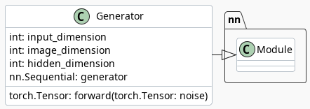
The Generator
This is the Deep Convolutional GAN from before.
class Generator(nn.Module):
    """The DCGAN Generator

    Args:
       input_dim: the dimension of the input vector
       im_chan: the number of channels in the images, fitted for the dataset used
             (MNIST is black-and-white, so 1 channel is your default)
       hidden_dim: the inner dimension,
    """
    def __init__(self, z_dim: int=10, im_chan: int=1, hidden_dim: int=64):
        super().__init__()
        self.input_dim = input_dim

        self.gen = nn.Sequential(
            self.make_gen_block(input_dim, hidden_dim * 4),
            self.make_gen_block(hidden_dim * 4, hidden_dim * 2, kernel_size=4, stride=1),
            self.make_gen_block(hidden_dim * 2, hidden_dim),
            self.make_gen_block(hidden_dim, im_chan, kernel_size=4, final_layer=True),
        )

    def make_gen_block(self, input_channels: int, output_channels: int,
                       kernel_size: int=3, stride: int=2,
                       final_layer: bool=False) -> nn.Sequential:
        """Creates a block for the generator (sub sequence)

       The parts
        - a transposed convolution
        - a batchnorm (except for in the last layer)
        - an activation.

       Args:
           input_channels: how many channels the input feature representation has
           output_channels: how many channels the output feature representation should have
           kernel_size: the size of each convolutional filter, equivalent to (kernel_size, kernel_size)
           stride: the stride of the convolution
           final_layer: a boolean, true if it is the final layer and false otherwise
                     (affects activation and batchnorm)

       Returns:
        the sub-sequence of layers
       """

        if not final_layer:
            return nn.Sequential(
                nn.ConvTranspose2d(input_channels, output_channels, kernel_size, stride),
                nn.BatchNorm2d(output_channels),
                nn.ReLU(inplace=True),
            )
        else:
            return nn.Sequential(
                nn.ConvTranspose2d(input_channels, output_channels, kernel_size, stride),
                nn.Tanh(),
            )

    def forward(self, noise: torch.Tensor) -> torch.Tensor:
        """complete a forward pass of the generator: Given a noise tensor,

       Args:
        noise: a noise tensor with dimensions (n_samples, z_dim)

       Returns:
        generated images.
       """
        # unsqueeze the noise
        x = noise.view(len(noise), self.z_dim, 1, 1)
        return self.gen(x)
The Critic
This is also essentially the same as our Discriminator class from before.
class Critic(nn.Module):
    """
    Critic Class

    Args:
       im_chan: the number of channels in the images, fitted for the dataset used
             (MNIST is black-and-white, so 1 channel is your default)
       hidden_dim: the inner dimension
    """
    def __init__(self, im_chan: int=1, hidden_dim: int=64):
        super().__init__()
        self.crit = nn.Sequential(
            self.make_crit_block(im_chan, hidden_dim),
            self.make_crit_block(hidden_dim, hidden_dim * 2),
            self.make_crit_block(hidden_dim * 2, 1, final_layer=True),
        )

    def make_crit_block(self, input_channels: int, output_channels: int,
                        kernel_size: int=4, stride: int=2,
                        final_layer: bool=False) -> nn.Sequential:
        """Creates a sub-block for the network

        - a convolution
        - a batchnorm (except in the final layer)
        - an activation (except in the final layer).

       Args:
           input_channels: how many channels the input feature representation has
           output_channels: how many channels the output feature representation should have
           kernel_size: the size of each convolutional filter, equivalent to (kernel_size, kernel_size)
           stride: the stride of the convolution
           final_layer: a boolean, true if it is the final layer and false otherwise
                     (affects activation and batchnorm)
       """
        if not final_layer:
            return nn.Sequential(
                nn.Conv2d(input_channels, output_channels, kernel_size,
                          stride),
                nn.BatchNorm2d(output_channels),
                nn.LeakyReLU(0.2),
            )
        else:
            return nn.Sequential(
                nn.Conv2d(input_channels, output_channels, kernel_size,
                          stride),
            )

    def forward(self, image: torch.Tensor) -> torch.Tensor:
        """Run a forward pass of the critic

       Args:
           image: a flattened image tensor with dimension (im_chan)

       Returns:
        a 1-dimension tensor representing fake/real.
       """
        crit_pred = self.crit(image)
        return crit_pred.view(len(crit_pred), -1)
Training
Hyperparameters
As usual, we'll start by setting the parameters:
- nepochs: the number of times you iterate through the entire dataset when training
- zdim: the dimension of the noise vector
- displaystep: how often to display/visualize the images
- batchsize: the number of images per forward/backward pass
- lr: the learning rate
- beta1, beta2: the momentum terms
- clambda: weight of the gradient penalty
- critrepeats: number of times to update the critic per generator update - there are more details about this in the Putting It All Together section
- device: the device type
n_epochs = 100
z_dim = 64
display_step = 50
batch_size = 128
lr = 0.0002
beta_1 = 0.5
beta_2 = 0.999
c_lambda = 10
crit_repeats = 5
device = 'cuda'
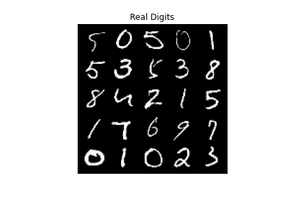
The Data
Once again we'll be using the MNIST dataset.
transform = transforms.Compose([
    transforms.ToTensor(),
    transforms.Normalize((0.5,), (0.5,)),
])

data_path = Path("~/pytorch-data/MNIST/").expanduser()
dataloader = DataLoader(
    MNIST(data_path, download=True, transform=transform),
    batch_size=batch_size,
    shuffle=True)
Setup For Training
gen = Generator(z_dim).to(device)
gen_opt = torch.optim.Adam(gen.parameters(), lr=lr, betas=(beta_1, beta_2))
crit = Critic().to(device)
crit_opt = torch.optim.Adam(crit.parameters(), lr=lr, betas=(beta_1, beta_2))
def weights_init(m):
    if isinstance(m, nn.Conv2d) or isinstance(m, nn.ConvTranspose2d):
        torch.nn.init.normal_(m.weight, 0.0, 0.02)
    if isinstance(m, nn.BatchNorm2d):
        torch.nn.init.normal_(m.weight, 0.0, 0.02)
        torch.nn.init.constant_(m.bias, 0)
    return
gen = gen.apply(weights_init)
crit = crit.apply(weights_init)
The Gradient
Calculating the gradient penalty can be broken into two functions: (1) compute the gradient with respect to the images and (2) compute the gradient penalty given the gradient.
You can start by getting the gradient. The gradient is computed by first creating a mixed image. This is done by weighing the fake and real image using epsilon and then adding them together. Once you have the intermediate image, you can get the critic's output on the image. Finally, you compute the gradient of the critic score's on the mixed images (output) with respect to the pixels of the mixed images (input).
def get_gradient(crit: Critic, real: torch.Tensor, fake: torch.Tensor,
                 epsilon: torch.Tensor) -> torch.tensor:
    """Gradient of the critic's scores with respect to mixes of real and fake images.

    Args:
       crit: the critic model
       real: a batch of real images
       fake: a batch of fake images
       epsilon: a vector of the uniformly random proportions of real/fake per mixed image

    Returns:
       gradient: the gradient of the critic's scores, with respect to the mixed image
    """
    # Mix the images together
    mixed_images = real * epsilon + fake * (1 - epsilon)

    # Calculate the critic's scores on the mixed images
    mixed_scores = crit(mixed_images)

    # Take the gradient of the scores with respect to the images
    gradient = torch.autograd.grad(
        # Note: You need to take the gradient of outputs with respect to inputs.
        #### START CODE HERE ####
        inputs = mixed_images,
        outputs = mixed_scores,
        #### END CODE HERE ####
        # These other parameters have to do with how the pytorch autograd engine works
        grad_outputs=torch.ones_like(mixed_scores),
        create_graph=True,
        retain_graph=True,
    )[0]
    return gradient
- Unit Tests
def test_get_gradient(image_shape):
    real = torch.randn(*image_shape, device=device) + 1
    fake = torch.randn(*image_shape, device=device) - 1
    epsilon_shape = [1 for _ in image_shape]
    epsilon_shape[0] = image_shape[0]
    epsilon = torch.rand(epsilon_shape, device=device).requires_grad_()
    gradient = get_gradient(crit, real, fake, epsilon)
    assert tuple(gradient.shape) == image_shape
    assert gradient.max() > 0
    assert gradient.min() < 0
    return gradient
gradient = test_get_gradient((256, 1, 28, 28))
The Gradient Penalty
The second function you need to complete is to compute the gradient penalty given the gradient. First, you calculate the magnitude of each image's gradient. The magnitude of a gradient is also called the norm. Then, you calculate the penalty by squaring the distance between each magnitude and the ideal norm of 1 and taking the mean of all the squared distances.
- Make sure you take the mean at the end.
- Note that the magnitude of each gradient has already been calculated for you.
def gradient_penalty(gradient: torch.Tensor) -> torch.Tensor:
    """Calculate the size of each image's gradient
    and penalize the mean quadratic distance of each magnitude to 1.

    Args:
       gradient: the gradient of the critic's scores, with respect to the mixed image

    Returns:
       penalty: the gradient penalty
    """
    # Flatten the gradients so that each row captures one image
    gradient = gradient.view(len(gradient), -1)

    # Calculate the magnitude of every row
    gradient_norm = gradient.norm(2, dim=1)

    # Penalize the mean squared distance of the gradient norms from 1
    penalty = torch.mean(torch.square(gradient_norm - 1))
    return penalty
- Unit Testing
def test_gradient_penalty(image_shape: tuple):
    bad_gradient = torch.zeros(*image_shape)
    bad_gradient_penalty = gradient_penalty(bad_gradient)
    assert torch.isclose(bad_gradient_penalty, torch.tensor(1.))

    image_size = torch.prod(torch.Tensor(image_shape[1:]))
    good_gradient = torch.ones(*image_shape) / torch.sqrt(image_size)
    good_gradient_penalty = gradient_penalty(good_gradient)
    assert torch.isclose(good_gradient_penalty, torch.tensor(0.))

    random_gradient = test_get_gradient(image_shape)
    random_gradient_penalty = gradient_penalty(random_gradient)
    assert torch.abs(random_gradient_penalty - 1) < 0.1
test_gradient_penalty((256, 1, 28, 28))
Losses
Next, you need to calculate the loss for the generator and the critic.
- Generator Loss
For the generator, the loss is calculated by maximizing the critic's prediction on the generator's fake images. The argument has the scores for all fake images in the batch, but you will use the mean of them.
- This can be written in one line.
- This is the negative of the mean of the critic's scores.
def get_gen_loss(crit_fake_pred: torch.Tensor) -> torch.Tensor:
    """loss of generator given critic's scores of generator's fake images.

    Args:
       crit_fake_pred: the critic's scores of the fake images

    Returns:
       gen_loss: a scalar loss value for the current batch of the generator
    """
    return -torch.mean(crit_fake_pred)
assert torch.isclose(
    get_gen_loss(torch.tensor(1.)), torch.tensor(-1.0)
)

assert torch.isclose(
    get_gen_loss(torch.rand(10000)), torch.tensor(-0.5), 0.05
)
- The Critic Loss
For the critic, the loss is calculated by maximizing the distance between the critic's predictions on the real images and the predictions on the fake images while also adding a gradient penalty. The gradient penalty is weighed according to lambda. The arguments are the scores for all the images in the batch, and you will use the mean of them.
- The higher the mean fake score, the higher the critic's loss is.
- What does this suggest about the mean real score?
- The higher the gradient penalty, the higher the critic's loss is, proportional to lambda.
def get_crit_loss(crit_fake_pred: torch.Tensor, crit_real_pred: torch.Tensor,
                  gp: torch.Tensor, c_lambda: torch.Tensor) -> torch.Tensor:
    """loss of a critic given critic's scores for fake and real images,
    the gradient penalty, and gradient penalty weight.

    Args:
       crit_fake_pred: the critic's scores of the fake images
       crit_real_pred: the critic's scores of the real images
       gp: the unweighted gradient penalty
       c_lambda: the current weight of the gradient penalty

    Returns:
       crit_loss: a scalar for the critic's loss, accounting for the relevant factors
    """
    return torch.mean(crit_fake_pred - crit_real_pred  + gp * c_lambda)
assert torch.isclose(
    get_crit_loss(torch.tensor(1.), torch.tensor(2.), torch.tensor(3.), 0.1),
    torch.tensor(-0.7)
)
assert torch.isclose(
    get_crit_loss(torch.tensor(20.), torch.tensor(-20.), torch.tensor(2.), 10),
    torch.tensor(60.)
)
Running the Training
Before you put everything together, there are a few things to note.
- Even on GPU, the training will run more slowly than previous labs because the gradient penalty requires you to compute the gradient of a gradient – this means potentially a few minutes per epoch! For best results, run this for as long as you can while on GPU.
- One important difference from earlier versions is that you will update the critic multiple times every time you update the generator This helps prevent the generator from overpowering the critic. Sometimes, you might see the reverse, with the generator updated more times than the critic. This depends on architectural (e.g. the depth and width of the network) and algorithmic choices (e.g. which loss you're using).
- WGAN-GP isn't necessarily meant to improve overall performance of a GAN, but just increases stability and avoids mode collapse. In general, a WGAN will be able to train in a much more stable way than the vanilla DCGAN from last assignment, though it will generally run a bit slower. You should also be able to train your model for more epochs without it collapsing.
def update_critic(critic, critic_optimizer, generator, generator_optimizer, batch_size, z_dim, real):
    critic_optimizer.zero_grad()
    fake_noise = make_noise(batch_size, z_dim, device=device)
    fake = generator(fake_noise)
    crit_fake_pred = critic(fake.detach())
    crit_real_pred = critic(real)

    epsilon = torch.rand(len(real), 1, 1, 1, device=device, requires_grad=True)
    gradient = get_gradient(critic, real, fake.detach(), epsilon)
    gp = gradient_penalty(gradient)
    crit_loss = get_crit_loss(crit_fake_pred, crit_real_pred, gp, c_lambda)

    # Keep track of the average critic loss in this batch
    mean_iteration_critic_loss = crit_loss.detach().item() / crit_repeats
    # Update gradients
    crit_loss.backward()
    # Update optimizer
    crit_opt.step()
    return mean_iteration_critic_loss, fake
def update_generator(generator, generator_optimizer, critic, critic_optimizer,
                     batch_size, z_dim):
        generator_optimizer.zero_grad()
        fake_noise_2 = make_noise(batch_size, z_dim, device=device)
        fake_2 = generator(fake_noise_2)
        crit_fake_pred = critic(fake_2)

        gen_loss = get_gen_loss(crit_fake_pred)
        gen_loss.backward()

        # Update the weights
        generator_optimizer.step()
        return [gen_loss.detach().item()]
cur_step = 0
generator_losses = []
critic_losses = []
fakes = []

with TIMER:
    for epoch in range(n_epochs):
        # Dataloader returns the batches
        for real, _ in dataloader:
            cur_batch_size = len(real)
            real = real.to(device)

            mean_iteration_critic_loss = 0
            for _ in range(crit_repeats):
                ### Update critic ###
                this_loss, fake = update_critic(crit, crit_opt, gen, gen_opt,
                                                cur_batch_size, z_dim, real)
                mean_iteration_critic_loss += this_loss
            critic_losses += [mean_iteration_critic_loss]

            ### Update generator ###
            # Keep track of the average generator loss
            generator_losses += update_generator(gen, gen_opt, crit, crit_opt,
                                                 cur_batch_size, z_dim)

            ### Visualization code ###
            if cur_step % display_step == 0 and cur_step > 0:
                gen_mean = sum(generator_losses[-display_step:]) / display_step
                crit_mean = sum(critic_losses[-display_step:]) / display_step
                print(f"Step {cur_step}: Generator loss: {gen_mean}, critic loss: {crit_mean}")
                fakes.append(fake)
                #show_tensor_images(fake)
                # show_tensor_images(real)
                # step_bins = 20
                #num_examples = (len(generator_losses) // step_bins) * step_bins
                #plt.plot(
                #    range(num_examples // step_bins),
                #    torch.Tensor(generator_losses[:num_examples]).view(-1, step_bins).mean(1),
                #    label="Generator Loss"
                #)
                #plt.plot(
                #    range(num_examples // step_bins),
                #    torch.Tensor(critic_losses[:num_examples]).view(-1, step_bins).mean(1),
                #    label="Critic Loss"
                #)
                #plt.legend()
                #plt.show()

            cur_step += 1
Started: 2021-04-23 16:44:37.086571
Step 50: Generator loss: 1.2940945455431938, critic loss: -2.5389487731456755
Step 100: Generator loss: 1.8233803486824036, critic loss: -10.170887191772463
Step 150: Generator loss: -0.8236922709643841, critic loss: -25.889275665283208
Step 200: Generator loss: -1.9489177632331849, critic loss: -57.93669644165039
Step 250: Generator loss: -1.6910316547751427, critic loss: -98.02721130371094
Step 300: Generator loss: -1.057899413406849, critic loss: -148.77607403564457
Step 350: Generator loss: -1.0930944073200226, critic loss: -199.94886077880858
Step 400: Generator loss: 1.900166620016098, critic loss: -245.53067184448247
Step 450: Generator loss: -18.928784263134002, critic loss: -251.46439450645448
Step 500: Generator loss: -7.688082475662231, critic loss: -289.45334830856325
Step 550: Generator loss: 12.447209596633911, critic loss: -395.351733947754
Step 600: Generator loss: 4.604712443947792, critic loss: -442.96986193847647
Step 650: Generator loss: 2.1788939160108565, critic loss: -480.044010131836
Step 700: Generator loss: 2.979072951376438, critic loss: -519.4769331054689
Step 750: Generator loss: -49.77768729448319, critic loss: -406.99980457305907
Step 800: Generator loss: 0.28986886143684387, critic loss: -444.8244698066711
Step 850: Generator loss: 31.1217813873291, critic loss: -608.1500103759765
Step 900: Generator loss: 12.006675623655319, critic loss: -632.0770750808719
Step 950: Generator loss: -0.15041383981704712, critic loss: -659.3277660064699
Step 1000: Generator loss: 15.936325817108154, critic loss: -629.952421447754
Step 1050: Generator loss: -43.25309041261673, critic loss: -504.54743419075004
Step 1100: Generator loss: -127.80617136001587, critic loss: -347.7993973159789
Step 1150: Generator loss: 4.186352119445801, critic loss: -461.6966292152405
Step 1200: Generator loss: 19.471285017728807, critic loss: -417.6742295103073
Step 1250: Generator loss: 34.04052387237549, critic loss: -327.74495936584475
Step 1300: Generator loss: -61.267093954086306, critic loss: -114.96264076042176
Step 1350: Generator loss: -56.96540081501007, critic loss: -257.8397505912781
Step 1400: Generator loss: -58.51407446861267, critic loss: -284.2404485015868
Step 1450: Generator loss: -31.23556293010712, critic loss: -282.15282668590544
Step 1500: Generator loss: 21.97936663866043, critic loss: -201.8184239835738
Step 1550: Generator loss: -35.051265001297, critic loss: -268.2542330398559
Step 1600: Generator loss: -13.768656857013703, critic loss: -201.92625104904172
Step 1650: Generator loss: 22.134875717163087, critic loss: -222.15251140356065
Step 1700: Generator loss: -33.80421092987061, critic loss: -196.00927429389947
Step 1750: Generator loss: -57.25435597419739, critic loss: -182.85244289588928
Step 1800: Generator loss: -41.60410815238953, critic loss: -213.254286611557
Step 1850: Generator loss: -4.978743267059326, critic loss: -101.88668561553959
Step 1900: Generator loss: 43.375376815795896, critic loss: 24.468120357513428
Step 1950: Generator loss: 37.55927352905273, critic loss: 19.142875072479246
Step 2000: Generator loss: 30.793880767822266, critic loss: 27.632160606384268
Step 2050: Generator loss: 28.9916410446167, critic loss: 37.41749234771728
Step 2100: Generator loss: 28.57459102630615, critic loss: 36.46667390441895
Step 2150: Generator loss: 27.179994583129883, critic loss: 37.36057964324953
Step 2200: Generator loss: 26.722407608032228, critic loss: 36.42123816680908
Step 2250: Generator loss: 26.215636711120606, critic loss: 35.10568865203857
Step 2300: Generator loss: 25.28977954864502, critic loss: 38.4949776916504
Step 2350: Generator loss: 25.161714172363283, critic loss: 30.91700393295288
Step 2400: Generator loss: 25.609521713256836, critic loss: 27.127794273376463
Step 2450: Generator loss: 26.457210426330565, critic loss: 23.25596778869629
Step 2500: Generator loss: 27.144473686218262, critic loss: 18.423582084655763
Step 2550: Generator loss: 28.104863624572754, critic loss: 16.720462280273438
Step 2600: Generator loss: 29.460466690063477, critic loss: 13.846090631484987
Step 2650: Generator loss: 31.16196632385254, critic loss: 10.717047594070436
Step 2700: Generator loss: 32.86851013183594, critic loss: 8.973742393493652
Step 2750: Generator loss: 33.90616256713867, critic loss: 9.844469717025756
Step 2800: Generator loss: 34.65669334411621, critic loss: 8.557393852233888
Step 2850: Generator loss: 35.84923110961914, critic loss: 6.227309632301333
Step 2900: Generator loss: 37.1290372467041, critic loss: 4.664727992773057
Step 2950: Generator loss: 39.00773422241211, critic loss: 3.6960949053764343
Step 3000: Generator loss: 41.04932693481445, critic loss: 3.064339481592179
Step 3050: Generator loss: 43.54303398132324, critic loss: 1.5976664029359815
Step 3100: Generator loss: 46.25879165649414, critic loss: 0.43558707976341254
Step 3150: Generator loss: 48.358483200073245, critic loss: -0.8735819962918758
Step 3200: Generator loss: 49.9193138885498, critic loss: -1.9399951877593993
Step 3250: Generator loss: 50.604149169921875, critic loss: -2.96596682035923
Step 3300: Generator loss: 51.37260269165039, critic loss: -4.266795755624772
Step 3350: Generator loss: 50.53414665222168, critic loss: -6.2572406907081595
Step 3400: Generator loss: 49.34995780944824, critic loss: -8.031075536847114
Step 3450: Generator loss: 46.14337966918945, critic loss: -8.019683789610863
Step 3500: Generator loss: 42.769298782348635, critic loss: -9.498445952415468
Step 3550: Generator loss: 37.38293798446655, critic loss: -9.02791331624985
Step 3600: Generator loss: 32.84453460693359, critic loss: -9.934100509524345
Step 3650: Generator loss: 29.88087886810303, critic loss: -9.069164658904075
Step 3700: Generator loss: 27.295934791564942, critic loss: -12.109804625511167
Step 3750: Generator loss: 23.694135398864745, critic loss: -14.327697192192076
Step 3800: Generator loss: 22.836445541381835, critic loss: -15.450897558450697
Step 3850: Generator loss: 21.66964967727661, critic loss: -18.371595690727236
Step 3900: Generator loss: 22.644691734313966, critic loss: -18.472765784740442
Step 3950: Generator loss: 23.275020160675048, critic loss: -14.622903740763663
Step 4000: Generator loss: 20.404177145957945, critic loss: -20.265531128883364
Step 4050: Generator loss: 20.57322360277176, critic loss: -22.811122689247135
Step 4100: Generator loss: 20.653975734710695, critic loss: -21.081045699119564
Step 4150: Generator loss: 22.07396845817566, critic loss: -25.1140656299591
Step 4200: Generator loss: 23.147041385173797, critic loss: -25.637423175573346
Step 4250: Generator loss: 24.7466512966156, critic loss: -27.446938713431358
Step 4300: Generator loss: 23.155011949539183, critic loss: -29.866371290445326
Step 4350: Generator loss: 28.670740413665772, critic loss: -27.526438851594932
Step 4400: Generator loss: 28.197952184677124, critic loss: -32.777981144189845
Step 4450: Generator loss: 30.352355518341064, critic loss: -27.1594803442955
Step 4500: Generator loss: 28.54464930534363, critic loss: -33.94081681919097
Step 4550: Generator loss: 30.315768175125122, critic loss: -32.86432695555688
Step 4600: Generator loss: 31.542511186599732, critic loss: -30.20407930350304
Step 4650: Generator loss: 32.1046596121788, critic loss: -25.409390352845193
Step 4700: Generator loss: 32.14258025169372, critic loss: -31.69375462341309
Step 4750: Generator loss: 34.99601099014282, critic loss: -17.207461384415634
Step 4800: Generator loss: 34.72456073760986, critic loss: -28.68983098757266
Step 4850: Generator loss: 43.15867195129395, critic loss: -3.741025509417056
Step 4900: Generator loss: 39.205870933532715, critic loss: -10.995340047717095
Step 4950: Generator loss: 33.214964599609374, critic loss: -22.35341439080238
Step 5000: Generator loss: 36.83505029678345, critic loss: -22.059852074146274
Step 5050: Generator loss: 44.310142288208006, critic loss: -9.833503689646719
Step 5100: Generator loss: 46.455570983886716, critic loss: -6.97827914196253
Step 5150: Generator loss: 50.3965446472168, critic loss: 2.86564082187414
Step 5200: Generator loss: 49.87795219421387, critic loss: -1.3452879690229889
Step 5250: Generator loss: 47.53674819946289, critic loss: -2.096805039405823
Step 5300: Generator loss: 46.8746314239502, critic loss: -3.2593628435134883
Step 5350: Generator loss: 45.44812057495117, critic loss: -8.15779336643219
Step 5400: Generator loss: 44.419895820617675, critic loss: -14.570247013330457
Step 5450: Generator loss: 46.02410781860352, critic loss: -15.177982830524446
Step 5500: Generator loss: 49.54875686645508, critic loss: -9.89209368979931
Step 5550: Generator loss: 48.06167510986328, critic loss: -14.110691767692567
Step 5600: Generator loss: 49.201857833862306, critic loss: -14.137419148623945
Step 5650: Generator loss: 50.152088012695316, critic loss: -12.306397112727165
Step 5700: Generator loss: 48.29638786315918, critic loss: -16.661144974470133
Step 5750: Generator loss: 48.57353067398071, critic loss: -14.890159791767603
Step 5800: Generator loss: 49.75064552307129, critic loss: -18.844482659339906
Step 5850: Generator loss: 60.04904914855957, critic loss: -6.717597324132919
Step 5900: Generator loss: 51.537723999023434, critic loss: -16.97626993632317
Step 5950: Generator loss: 53.64197952270508, critic loss: -17.934735801696778
Step 6000: Generator loss: 58.61811660766602, critic loss: -12.544874910593034
Step 6050: Generator loss: 57.9530167388916, critic loss: -12.869983579158779
Step 6100: Generator loss: 58.112417755126955, critic loss: -14.860800614833833
Step 6150: Generator loss: 59.45550857543945, critic loss: -16.21854728984833
Step 6200: Generator loss: 61.55990020751953, critic loss: -13.752459713578226
Step 6250: Generator loss: 63.91949012756348, critic loss: -15.32866345870495
Step 6300: Generator loss: 61.11529357910156, critic loss: -19.138810309529305
Step 6350: Generator loss: 68.78476165771484, critic loss: -3.858711770117282
Step 6400: Generator loss: 72.07508163452148, critic loss: -3.3317795319557204
Step 6450: Generator loss: 62.11038558959961, critic loss: -12.74781008577347
Step 6500: Generator loss: 66.10368064880372, critic loss: -13.66576182627678
Step 6550: Generator loss: 62.73857864379883, critic loss: -19.79733684468269
Step 6600: Generator loss: 64.86283889770507, critic loss: -15.91535943055153
Step 6650: Generator loss: 65.02771781921386, critic loss: -16.515603628635407
Step 6700: Generator loss: 73.10651649475098, critic loss: -7.974747009277344
Step 6750: Generator loss: 69.39200439453126, critic loss: -12.647881946563723
Step 6800: Generator loss: 70.61859390258789, critic loss: -14.981548887073998
Step 6850: Generator loss: 71.39209846496583, critic loss: -12.02037605035305
Step 6900: Generator loss: 68.91642692565918, critic loss: -17.377452049493794
Step 6950: Generator loss: 73.83714424133301, critic loss: -14.842290714025498
Step 7000: Generator loss: 76.0492682647705, critic loss: -4.022153543114662
Step 7050: Generator loss: 73.60314575195312, critic loss: -11.167652189731598
Step 7100: Generator loss: 73.69744178771973, critic loss: -16.215790304422377
Step 7150: Generator loss: 73.02161018371582, critic loss: -11.844917020320892
Step 7200: Generator loss: 84.43860961914062, critic loss: -4.338678442955016
Step 7250: Generator loss: 72.4216611480713, critic loss: -16.95018665671349
Step 7300: Generator loss: 75.08161041259766, critic loss: -13.94019952297211
Step 7350: Generator loss: 76.7044221496582, critic loss: -14.254385577440262
Step 7400: Generator loss: 81.03584564208984, critic loss: -3.171723330259324
Step 7450: Generator loss: 80.19454528808593, critic loss: -6.323260527610778
Step 7500: Generator loss: 74.55620361328126, critic loss: -8.62027923491597
Step 7550: Generator loss: 84.05591217041015, critic loss: -3.5706960783004775
Step 7600: Generator loss: 81.2258724975586, critic loss: -8.142396178722382
Step 7650: Generator loss: 73.19812255859375, critic loss: -16.196065732836722
Step 7700: Generator loss: 74.52944702148437, critic loss: -15.7419521817565
Step 7750: Generator loss: 80.32163719177247, critic loss: -7.413010147571564
Step 7800: Generator loss: 76.99493499755859, critic loss: -12.079633572757244
Step 7850: Generator loss: 81.32430145263672, critic loss: -2.8193510160446174
Step 7900: Generator loss: 80.63022003173828, critic loss: -3.1151746976375576
Step 7950: Generator loss: 75.89005561828613, critic loss: -8.688790566921234
Step 8000: Generator loss: 72.94720428466798, critic loss: -14.186805599212649
Step 8050: Generator loss: 80.84135955810547, critic loss: -11.586392744839191
Step 8100: Generator loss: 79.48079322814941, critic loss: -1.3788062819838527
Step 8150: Generator loss: 72.63796539306641, critic loss: -14.767250993669036
Step 8200: Generator loss: 76.29679145812989, critic loss: -16.04671211397648
Step 8250: Generator loss: 72.60974617004395, critic loss: -17.008654308915133
Step 8300: Generator loss: 75.25621772766114, critic loss: -12.109682399034496
Step 8350: Generator loss: 81.09654647827148, critic loss: -10.706179085254668
Step 8400: Generator loss: 77.28005485534668, critic loss: -4.09239830350876
Step 8450: Generator loss: 83.45014526367187, critic loss: -3.1862959499359125
Step 8500: Generator loss: 80.24715942382812, critic loss: -4.144565615177154
Step 8550: Generator loss: 76.43464157104492, critic loss: -9.53649512773752
Step 8600: Generator loss: 73.67140350341796, critic loss: -15.18680296653509
Step 8650: Generator loss: 75.6114599609375, critic loss: -10.128391755342484
Step 8700: Generator loss: 73.68272163391113, critic loss: -16.97586714470387
Step 8750: Generator loss: 83.1702619934082, critic loss: -0.6609140309095384
Step 8800: Generator loss: 80.41752578735351, critic loss: -4.212692310333251
Step 8850: Generator loss: 71.03237358093261, critic loss: -14.983835175275805
Step 8900: Generator loss: 75.80495880126954, critic loss: -12.667168443322183
Step 8950: Generator loss: 81.14228034973145, critic loss: 2.7472501730918872
Step 9000: Generator loss: 81.20193344116211, critic loss: -3.052738008499146
Step 9050: Generator loss: 73.43904174804688, critic loss: -7.423715700268742
Step 9100: Generator loss: 73.12181861877441, critic loss: -14.306883191585541
Step 9150: Generator loss: 76.89906158447266, critic loss: -13.396733086347583
Step 9200: Generator loss: 75.99712623596191, critic loss: -12.318668732821939
Step 9250: Generator loss: 77.78204513549805, critic loss: -6.621456883490087
Step 9300: Generator loss: 77.82661689758301, critic loss: -11.999425900220869
Step 9350: Generator loss: 81.48483535766601, critic loss: -11.480147421479224
Step 9400: Generator loss: 75.37383903503418, critic loss: -11.605070021390913
Step 9450: Generator loss: 83.24758972167969, critic loss: -1.770111013114451
Step 9500: Generator loss: 75.71745803833008, critic loss: -14.370290687352417
Step 9550: Generator loss: 80.75228134155273, critic loss: -12.244659341961144
Step 9600: Generator loss: 80.36522689819336, critic loss: -9.994889120757579
Step 9650: Generator loss: 79.76879989624024, critic loss: -12.11628355455398
Step 9700: Generator loss: 75.03965270996093, critic loss: -15.582087687492374
Step 9750: Generator loss: 78.26055725097656, critic loss: -9.227732668161394
Step 9800: Generator loss: 86.73946716308593, critic loss: -3.9114915781021113
Step 9850: Generator loss: 77.57634506225585, critic loss: -16.903033419966697
Step 9900: Generator loss: 79.62038360595703, critic loss: -13.387711975812913
Step 9950: Generator loss: 83.48049461364747, critic loss: 0.4212318459749224
Step 10000: Generator loss: 86.0385548400879, critic loss: -3.0202082567214954
Step 10050: Generator loss: 84.96556030273437, critic loss: -3.2984186277389527
Step 10100: Generator loss: 82.55163467407226, critic loss: -5.651416356563568
Step 10150: Generator loss: 72.47459297180175, critic loss: -16.2935069770813
Step 10200: Generator loss: 77.47050117492675, critic loss: -14.219993201971054
Step 10250: Generator loss: 82.40048095703125, critic loss: -9.951535837292676
Step 10300: Generator loss: 78.51686393737793, critic loss: -5.037457182884218
Step 10350: Generator loss: 79.00918548583985, critic loss: -10.983480290770531
Step 10400: Generator loss: 79.10479446411132, critic loss: -11.458023426651957
Step 10450: Generator loss: 79.01952590942383, critic loss: -13.550984252214432
Step 10500: Generator loss: 79.7324333190918, critic loss: -15.04755926167965
Step 10550: Generator loss: 83.25529792785645, critic loss: -10.678096773743627
Step 10600: Generator loss: 78.7729409790039, critic loss: -14.363517974853519
Step 10650: Generator loss: 83.80620101928712, critic loss: -12.4009742795825
Step 10700: Generator loss: 83.44554489135743, critic loss: -5.4632708239853365
Step 10750: Generator loss: 84.38950912475586, critic loss: -4.946207571595907
Step 10800: Generator loss: 84.90599151611327, critic loss: -10.688541789770127
Step 10850: Generator loss: 80.39469886779786, critic loss: -13.391746405303474
Step 10900: Generator loss: 79.68403381347656, critic loss: -14.792330410242082
Step 10950: Generator loss: 84.55435623168945, critic loss: -12.792006389081477
Step 11000: Generator loss: 85.3377848815918, critic loss: -1.002582928955554
Step 11050: Generator loss: 76.42176498413086, critic loss: -16.618346381425855
Step 11100: Generator loss: 82.8500619506836, critic loss: -10.213502784013746
Step 11150: Generator loss: 80.111083984375, critic loss: -16.506468793153765
Step 11200: Generator loss: 81.84511749267578, critic loss: -14.588824108004571
Step 11250: Generator loss: 82.36108421325683, critic loss: -14.826971750736238
Step 11300: Generator loss: 82.89525245666503, critic loss: -14.743118989944467
Step 11350: Generator loss: 78.9609211730957, critic loss: -6.072368972778322
Step 11400: Generator loss: 79.75704879760742, critic loss: -11.66915795624256
Step 11450: Generator loss: 92.73718231201173, critic loss: -8.626956017732619
Step 11500: Generator loss: 76.74110557556152, critic loss: -13.485125755786896
Step 11550: Generator loss: 86.92150177001953, critic loss: -11.96049699956179
Step 11600: Generator loss: 87.94025703430175, critic loss: -7.829241111636162
Step 11650: Generator loss: 78.58638778686523, critic loss: -13.818019400000573
Step 11700: Generator loss: 82.94163925170898, critic loss: -16.088717435359957
Step 11750: Generator loss: 82.20194442749023, critic loss: -13.443735618114472
Step 11800: Generator loss: 77.3590771484375, critic loss: -0.26538432469963885
Step 11850: Generator loss: 87.65712219238281, critic loss: -2.2925723257064816
Step 11900: Generator loss: 86.44266906738281, critic loss: -2.755362086296081
Step 11950: Generator loss: 85.7614064025879, critic loss: -2.9416364326477047
Step 12000: Generator loss: 84.22476821899414, critic loss: -3.100327790260315
Step 12050: Generator loss: 81.84705871582031, critic loss: -3.3889783926010137
Step 12100: Generator loss: 74.62463600158691, critic loss: -9.155223772525787
Step 12150: Generator loss: 83.41003746032715, critic loss: -7.312069640517238
Step 12200: Generator loss: 77.82574188232422, critic loss: -10.063361536026001
Step 12250: Generator loss: 77.09058532714843, critic loss: -15.389594004154203
Step 12300: Generator loss: 85.65135437011719, critic loss: -11.597671725511553
Step 12350: Generator loss: 79.91491325378418, critic loss: -0.8456090040206905
Step 12400: Generator loss: 83.31446044921876, critic loss: -3.5672192862033842
Step 12450: Generator loss: 80.4154541015625, critic loss: -9.493659735798834
Step 12500: Generator loss: 77.22660888671875, critic loss: -11.343838263094426
Step 12550: Generator loss: 76.51863540649414, critic loss: -15.957162732720372
Step 12600: Generator loss: 71.82434341430664, critic loss: -15.232202378749843
Step 12650: Generator loss: 81.55846801757812, critic loss: -12.02893185913563
Step 12700: Generator loss: 77.01351791381836, critic loss: -14.394531373143197
Step 12750: Generator loss: 82.79933059692382, critic loss: -10.995534277558324
Step 12800: Generator loss: 80.33022705078125, critic loss: -7.422801446437835
Step 12850: Generator loss: 77.88019416809082, critic loss: -10.48680070441961
Step 12900: Generator loss: 77.28355583190918, critic loss: -15.062006795048712
Step 12950: Generator loss: 72.02762420654297, critic loss: -18.125201426446434
Step 13000: Generator loss: 78.97825164794922, critic loss: -11.02606911355257
Step 13050: Generator loss: 76.02745002746582, critic loss: -13.242777463912965
Step 13100: Generator loss: 82.44893028259277, critic loss: -10.203380972802634
Step 13150: Generator loss: 80.63447105407715, critic loss: -11.436619911789894
Step 13200: Generator loss: 69.52673934936523, critic loss: -12.998723325610163
Step 13250: Generator loss: 75.26367416381837, critic loss: -12.58380482053757
Step 13300: Generator loss: 78.29216751098633, critic loss: 0.21028297042846839
Step 13350: Generator loss: 70.94842475891113, critic loss: -8.405993442416191
Step 13400: Generator loss: 77.60350791931153, critic loss: -12.201066960632803
Step 13450: Generator loss: 78.38650337219238, critic loss: -13.255251537919046
Step 13500: Generator loss: 72.39071220397949, critic loss: -13.91472595399618
Step 13550: Generator loss: 78.81595336914063, critic loss: -12.717635474145416
Step 13600: Generator loss: 69.23250061035156, critic loss: -15.01334501111508
Step 13650: Generator loss: 77.3666291809082, critic loss: -16.321711009979246
Step 13700: Generator loss: 73.45859939575195, critic loss: -17.17580293393135
Step 13750: Generator loss: 74.07134948730469, critic loss: -14.143001305580142
Step 13800: Generator loss: 68.98319381713867, critic loss: -18.013431072473526
Step 13850: Generator loss: 73.18379371643067, critic loss: -13.245033169150352
Step 13900: Generator loss: 73.70108238220215, critic loss: -15.747089947700497
Step 13950: Generator loss: 71.67143341064452, critic loss: -6.442092946648602
Step 14000: Generator loss: 74.99322380065918, critic loss: -5.310949310302733
Step 14050: Generator loss: 69.55456466674805, critic loss: -7.584069814443586
Step 14100: Generator loss: 68.11343818664551, critic loss: -15.932588892817499
Step 14150: Generator loss: 73.32868095397949, critic loss: -14.538219540774824
Step 14200: Generator loss: 71.54050506591797, critic loss: -6.507004916965961
Step 14250: Generator loss: 73.50055587768554, critic loss: -12.074983437180519
Step 14300: Generator loss: 75.37609176635742, critic loss: -12.215355042934414
Step 14350: Generator loss: 78.41978523254394, critic loss: -13.282461894750588
Step 14400: Generator loss: 69.06725090026856, critic loss: -8.44315874606371
Step 14450: Generator loss: 77.47375007629394, critic loss: -10.59642046368122
Step 14500: Generator loss: 72.112548828125, critic loss: -9.080148652315138
Step 14550: Generator loss: 71.41747200012207, critic loss: -12.610691975355143
Step 14600: Generator loss: 68.53853507995605, critic loss: -14.517420025825501
Step 14650: Generator loss: 71.00217765808105, critic loss: -16.055311642885208
Step 14700: Generator loss: 75.56183944702148, critic loss: -4.261986103117466
Step 14750: Generator loss: 68.21860916137695, critic loss: -14.03696541213989
Step 14800: Generator loss: 71.7959959411621, critic loss: -13.989702057063587
Step 14850: Generator loss: 76.38227409362793, critic loss: -10.939811514139176
Step 14900: Generator loss: 67.81556015014648, critic loss: -15.070325279712678
Step 14950: Generator loss: 71.62906150817871, critic loss: -12.239016912937165
Step 15000: Generator loss: 73.60893783569335, critic loss: -5.476252611890436
Step 15050: Generator loss: 64.43828086853027, critic loss: -11.680644391536712
Step 15100: Generator loss: 66.76135398864746, critic loss: -18.935012437820443
Step 15150: Generator loss: 64.45999412536621, critic loss: -16.77594568133354
Step 15200: Generator loss: 68.81907485961914, critic loss: -16.819265387773513
Step 15250: Generator loss: 71.44663459777831, critic loss: -14.780536164999004
Step 15300: Generator loss: 69.05639785766601, critic loss: -15.773872276782981
Step 15350: Generator loss: 72.00610313415527, critic loss: -12.428475862145426
Step 15400: Generator loss: 66.33817840576172, critic loss: -11.460507846534249
Step 15450: Generator loss: 73.98657371520996, critic loss: -12.046799251675607
Step 15500: Generator loss: 71.14604766845703, critic loss: -14.48868891143799
Step 15550: Generator loss: 72.55676879882813, critic loss: -9.285633412837981
Step 15600: Generator loss: 72.27706947326661, critic loss: -11.433179477930068
Step 15650: Generator loss: 70.14899436950684, critic loss: -14.64919223260879
Step 15700: Generator loss: 70.52759353637695, critic loss: -13.822800672113893
Step 15750: Generator loss: 66.5163092803955, critic loss: -13.497988208055496
Step 15800: Generator loss: 65.68713722229003, critic loss: -13.090139507174491
Step 15850: Generator loss: 68.86076667785645, critic loss: -12.112882311582563
Step 15900: Generator loss: 72.71573020935058, critic loss: -11.739855915784835
Step 15950: Generator loss: 69.23649925231933, critic loss: 1.5610642746686931
Step 16000: Generator loss: 63.27606719970703, critic loss: -6.625546929836272
Step 16050: Generator loss: 65.96758232116699, critic loss: -17.750343059539794
Step 16100: Generator loss: 62.09547576904297, critic loss: -17.4672027888298
Step 16150: Generator loss: 75.76868995666504, critic loss: -12.86666469740868
Step 16200: Generator loss: 64.08884880065918, critic loss: -7.587684287369252
Step 16250: Generator loss: 64.09755882263184, critic loss: -10.57423495966196
Step 16300: Generator loss: 66.86840660095214, critic loss: -3.5877239196300508
Step 16350: Generator loss: 70.60188285827637, critic loss: -7.692209842979907
Step 16400: Generator loss: 62.29129165649414, critic loss: -12.677523095130923
Step 16450: Generator loss: 62.98073165893555, critic loss: -13.866112356960771
Step 16500: Generator loss: 61.780632400512694, critic loss: -6.281874860048294
Step 16550: Generator loss: 62.74724609375, critic loss: -13.956338333368299
Step 16600: Generator loss: 61.48925178527832, critic loss: -16.810678883075717
Step 16650: Generator loss: 52.7329150390625, critic loss: -18.111987345457074
Step 16700: Generator loss: 60.26760322570801, critic loss: -17.837719259858133
Step 16750: Generator loss: 60.27441291809082, critic loss: -14.668455944180492
Step 16800: Generator loss: 64.81710945129394, critic loss: -8.937785160303115
Step 16850: Generator loss: 61.87463485717773, critic loss: -13.174851733446122
Step 16900: Generator loss: 66.52726516723632, critic loss: -17.641908020138743
Step 16950: Generator loss: 63.35795883178711, critic loss: -17.725372922539712
Step 17000: Generator loss: 67.46929817199707, critic loss: -13.343407141447067
Step 17050: Generator loss: 59.79177055358887, critic loss: -16.512492282271385
Step 17100: Generator loss: 66.42052528381348, critic loss: -9.183917128443717
Step 17150: Generator loss: 59.208996353149416, critic loss: -13.243339603602893
Step 17200: Generator loss: 63.88817520141602, critic loss: -13.442776112914084
Step 17250: Generator loss: 69.03452033996582, critic loss: -11.0614826682806
Step 17300: Generator loss: 57.58331108093262, critic loss: -13.529039879202841
Step 17350: Generator loss: 67.6368569946289, critic loss: -11.620229701399802
Step 17400: Generator loss: 60.044710845947264, critic loss: -9.055887681692841
Step 17450: Generator loss: 64.43620628356933, critic loss: -11.920627628207207
Step 17500: Generator loss: 56.046851272583005, critic loss: -22.301562000870714
Step 17550: Generator loss: 62.282958908081056, critic loss: -14.955312865734099
Step 17600: Generator loss: 65.897964553833, critic loss: -6.340100202620029
Step 17650: Generator loss: 58.14865257263184, critic loss: -10.649906709671022
Step 17700: Generator loss: 66.7437523651123, critic loss: -12.996105446338657
Step 17750: Generator loss: 63.59517837524414, critic loss: -12.67168800020218
Step 17800: Generator loss: 65.87414787292481, critic loss: -13.124171116769311
Step 17850: Generator loss: 66.03790901184082, critic loss: -13.294757736086847
Step 17900: Generator loss: 56.273787307739255, critic loss: -18.649981175422667
Step 17950: Generator loss: 68.3505224609375, critic loss: -13.77443748676777
Step 18000: Generator loss: 59.758854675292966, critic loss: -13.528435281991955
Step 18050: Generator loss: 70.61318840026856, critic loss: -12.014795050919052
Step 18100: Generator loss: 62.63155372619629, critic loss: -9.601117482304572
Step 18150: Generator loss: 58.44773849487305, critic loss: -9.71425095164776
Step 18200: Generator loss: 59.341090240478515, critic loss: -16.878086137115954
Step 18250: Generator loss: 57.848808708190916, critic loss: -19.507797758817674
Step 18300: Generator loss: 63.10433967590332, critic loss: -4.3734778246283526
Step 18350: Generator loss: 57.56446601867676, critic loss: -10.789146659135817
Step 18400: Generator loss: 51.76399398803711, critic loss: -15.076736944794657
Step 18450: Generator loss: 57.02366355895996, critic loss: -12.479052137970923
Step 18500: Generator loss: 62.833531875610355, critic loss: -12.99720428943634
Step 18550: Generator loss: 56.588841400146485, critic loss: -14.211519970417026
Step 18600: Generator loss: 61.620222854614255, critic loss: -14.894168957710265
Step 18650: Generator loss: 59.04514297485352, critic loss: -3.9987226614952096
Step 18700: Generator loss: 54.68501613616943, critic loss: -13.798751793980603
Step 18750: Generator loss: 60.477030181884764, critic loss: -13.97087904036045
Step 18800: Generator loss: 59.51054759979248, critic loss: -18.694762709856033
Step 18850: Generator loss: 53.82080192565918, critic loss: -14.210277070969342
Step 18900: Generator loss: 64.43251205444336, critic loss: -13.768319549560543
Step 18950: Generator loss: 56.9788289642334, critic loss: -10.571144456863403
Step 19000: Generator loss: 59.03595703125, critic loss: -12.603199533462528
Step 19050: Generator loss: 60.19775802612305, critic loss: -14.499388661146167
Step 19100: Generator loss: 59.592409973144534, critic loss: -8.202755635917187
Step 19150: Generator loss: 55.50546585083008, critic loss: -16.347688998579976
Step 19200: Generator loss: 61.19869083404541, critic loss: -18.950819284915923
Step 19250: Generator loss: 66.31558391571045, critic loss: -12.890463754177098
Step 19300: Generator loss: 57.29240139007568, critic loss: -18.10998232960701
Step 19350: Generator loss: 59.32999900817871, critic loss: -13.577078444600104
Step 19400: Generator loss: 65.96876052856446, critic loss: -11.8188825455904
Step 19450: Generator loss: 56.72755683898926, critic loss: -14.319641982913016
Step 19500: Generator loss: 57.38858169555664, critic loss: -17.450813733339313
Step 19550: Generator loss: 66.02516723632813, critic loss: -10.693548452854154
Step 19600: Generator loss: 54.7833975982666, critic loss: -13.142704640865325
Step 19650: Generator loss: 57.28132354736328, critic loss: -14.967523851156233
Step 19700: Generator loss: 59.98361915588379, critic loss: -16.183865994155408
Step 19750: Generator loss: 58.18478466033935, critic loss: -15.35918751955032
Step 19800: Generator loss: 63.54511661529541, critic loss: -10.502776491999626
Step 19850: Generator loss: 56.24938293457031, critic loss: -6.75664558506012
Step 19900: Generator loss: 60.40652961730957, critic loss: -13.489446130156516
Ended: 2021-04-23 17:33:03.659309
Elapsed: 0:48:26.572738
---------------------------------------------------------------------------
RuntimeError                              Traceback (most recent call last)
<ipython-input-35-08d8bddbdcc4> in <module>
     14             for _ in range(crit_repeats):
     15                 ### Update critic ###
---> 16                 this_loss, fake = update_critic(crit, crit_opt, gen, gen_opt,
     17                                                 cur_batch_size, z_dim, real)
     18                 mean_iteration_critic_loss += this_loss

<ipython-input-33-696fefd91963> in update_critic(critic, critic_optimizer, generator, generator_optimizer, batch_size, z_dim, real)
      7
      8     epsilon = torch.rand(len(real), 1, 1, 1, device=device, requires_grad=True)
----> 9     gradient = get_gradient(critic, real, fake.detach(), epsilon)
     10     gp = gradient_penalty(gradient)
     11     crit_loss = get_crit_loss(crit_fake_pred, crit_real_pred, gp, c_lambda)

<ipython-input-16-06dea6615386> in get_gradient(crit, real, fake, epsilon)
     19
     20     # Take the gradient of the scores with respect to the images
---> 21     gradient = torch.autograd.grad(
     22         # Note: You need to take the gradient of outputs with respect to inputs.
     23         #### START CODE HERE ####

~/.conda/envs/neurotic-pytorch/lib/python3.9/site-packages/torch/autograd/__init__.py in grad(outputs, inputs, grad_outputs, retain_graph, create_graph, only_inputs, allow_unused)
    221         retain_graph = create_graph
    222
--> 223     return Variable._execution_engine.run_backward(
    224         outputs, grad_outputs_, retain_graph, create_graph,
    225         inputs, allow_unused, accumulate_grad=False)

RuntimeError: CUDA out of memory. Tried to allocate 20.00 MiB (GPU 0; 7.92 GiB total capacity; 7.13 GiB already allocated; 24.62 MiB free; 7.13 GiB reserved in total by PyTorch)
End
- Arjovsky M, Chintala S, Bottou L. Wasserstein generative adversarial networks. International conference on machine learning 2017 Jul 17 (pp. 214-223). PMLR. (archiv.org)
- Gulrajani I, Ahmed F, Arjovsky M, Dumoulin V, Courville A. Improved training of wasserstein gans. arXiv preprint arXiv:1704.00028. 2017 Mar 31. (archiv.org)