1 Introduction

This looks at the performance of the K-Nearest Neighbors for classification. K-Nearest Neighbors works by finding the k (count) of neighbors that are closest to the data-point and classifying the point using the majority vote of those points. I'm going to use the default distance measurement of Euclidean distance. Fitting in this case means memorizing all the data so you can use it for predictions and then doing the calculations when you need to make a prediction. This makes it memory-intensive and slower when it's used to make predictions, so it's useful as a baseline, but not in production.

2 Synthetic

I'll start with a synthetic data set created by sklean. I'll make it the same shape as the Breast Cancer case that I'll look at later.

2.1 Imports

from sklearn.datasets import make_classification
from sklearn.model_selection import train_test_split
from sklearn.neighbors import KNeighborsClassifier
import matplotlib.pyplot as pyplot
import seaborn

%matplotlib inline
seaborn.set_style("whitegrid")

2.2 The Data

total = 569
positive_fraction = 212/total
negative_fraction = 1 - positive_fraction
inputs, classifications = make_classification(n_samples=total, n_features=30,
                                              weights=[positive_fraction,
                                                       negative_fraction])
print(inputs.shape)
print(classifications.shape)

(569, 30)
(569,)

positive = classifications.sum()
print("Positives: {}".format(positive))
print("Negatives: {}".format(classifications.size - positive))

Positives: 355
Negatives: 214

X_train, X_test, y_train, y_test = train_test_split(inputs, classifications)

2.3 The model

model = KNeighborsClassifier()

def get_accuracies(max_neighbors=10):
    train_accuracies = []
    test_accuracies = []
    for neighbors in range(1,  max_neighbors+1):
        classifier = KNeighborsClassifier(n_neighbors=neighbors)
        classifier.fit(X_train, y_train)
        train_accuracies.append(classifier.score(X_train, y_train))
        test_accuracies.append(classifier.score(X_test, y_test))
    return train_accuracies, test_accuracies

training_accuracies, testing_accuracies = get_accuracies()

neighbors = range(1, 11)
pyplot.plot(neighbors, training_accuracies, label="Training Accuracy")
pyplot.plot(neighbors, testing_accuracies, label="Testing Accuracy")
pyplot.ylabel("Accuracy")
pyplot.xlabel("Neighbors")
pyplot.title("KNN Cancer Accuracy")
pyplot.legend()

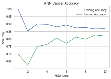
At k=1, the training set does perfectly while the test set does okay, but not as well as it does at k=9, what appears to be the best value.

3 Breast Cancer

3.1 Imports

import matplotlib.pyplot as pyplot
import seaborn
import pandas
from sklearn.model_selection import train_test_split
from sklearn.datasets import load_breast_cancer
from sklearn.neighbors import KNeighborsClassifier

%matplotlib inline
seaborn.set_style("whitegrid")

3.2 The Dataset

cancer = load_breast_cancer()
print("Keys in the cancer bunch: {}".format(",".join(cancer.keys())))
print("Training Data Shape: {}".format(cancer.data.shape))
print("Target Names: {}".format(','.join(cancer.target_names)))

Keys in the cancer bunch: feature_names,target_names,target,data,DESCR
Training Data Shape: (569, 30)
Target Names: malignant,benign

This is from the description.

Data Set Characteristics:

Number of Instances:
	569

Number of Attributes:
	30 numeric, predictive attributes and the class
Attribute Information:

radius (mean of distances from center to points on the perimeter)
texture (standard deviation of gray-scale values)
perimeter
area
smoothness (local variation in radius lengths)
compactness (perimeter^2 / area - 1.0)
concavity (severity of concave portions of the contour)
concave points (number of concave portions of the contour)
symmetry
fractal dimension ("coastline approximation" - 1)

The mean, standard error, and "worst" or largest (mean of the three largest values) of these features were computed for each image, resulting in 30 features. For instance, field 3 is Mean Radius, field 13 is Radius SE, field 23 is Worst Radius.

class:
- WDBC-Malignant
- WDBC-Benign

Missing Attribute Values:
	None
Class Distribution:
	212 - Malignant, 357 - Benign
Creator:	Dr. William H. Wolberg, W. Nick Street, Olvi L. Mangasarian
Donor:	Nick Street
Date:	November, 1995

This is a copy of UCI ML Breast Cancer Wisconsin (Diagnostic) datasets. https://goo.gl/U2Uwz2

Features are computed from a digitized image of a fine needle aspirate (FNA) of a breast mass. They describe characteristics of the cell nuclei present in the image.

Separating plane described above was obtained using Multisurface Method-Tree (MSM-T) [K. P. Bennett, "Decision Tree Construction Via Linear Programming." Proceedings of the 4th Midwest Artificial Intelligence and Cognitive Science Society, pp. 97-101, 1992], a classification method which uses linear programming to construct a decision tree. Relevant features were selected using an exhaustive search in the space of 1-4 features and 1-3 separating planes.

The actual linear program used to obtain the separating plane in the 3-dimensional space is that described in: [K. P. Bennett and O. L. Mangasarian: "Robust Linear Programming Discrimination of Two Linearly Inseparable Sets", Optimization Methods and Software 1, 1992, 23-34].

This database is also available through the UW CS ftp server:

ftp ftp.cs.wisc.edu cd math-prog/cpo-dataset/machine-learn/WDBC/

References

W.N. Street, W.H. Wolberg and O.L. Mangasarian. Nuclear feature extraction for breast tumor diagnosis. IS&T/SPIE 1993 International Symposium on Electronic Imaging: Science and Technology, volume 1905, pages 861-870, San Jose, CA, 1993.
O.L. Mangasarian, W.N. Street and W.H. Wolberg. Breast cancer diagnosis and prognosis via linear programming. Operations Research, 43(4), pages 570-577, July-August 1995.
W.H. Wolberg, W.N. Street, and O.L. Mangasarian. Machine learning techniques to diagnose breast cancer from fine-needle aspirates. Cancer Letters 77 (1994) 163-171.

Loading the Data

target = pandas.DataFrame(dict(target=cancer.target))
target_map = dict(zip(range(len(cancer.target_names)), cancer.target_names))
target['name'] = target.target.apply(lambda entry: target_map[entry])
print(target.name.value_counts())

benign       357
malignant    212
Name: name, dtype: int64

3.3 Splitting the Data

X_train, X_test, y_train, y_test = train_test_split(cancer.data, cancer.target, stratify=cancer.target)
print("Trainining percent: {0:.2f} %".format(100 * len(y_train)/len(cancer.target)))
print("Testing percent: {0:.2f}".format(100 * len(y_test)/len(cancer.target)))

Trainining percent: 74.87 %
Testing percent: 25.13

3.4 Model Performance

def get_accuracies(max_neighbors=10):
    train_accuracies = []
    test_accuracies = []
    for neighbors in range(1,  max_neighbors+1):
        classifier = KNeighborsClassifier(n_neighbors=neighbors)
        classifier.fit(X_train, y_train)
        train_accuracies.append(classifier.score(X_train, y_train))
        test_accuracies.append(classifier.score(X_test, y_test))
    return train_accuracies, test_accuracies

training_accuracies, testing_accuracies = get_accuracies()

neighbors = range(1, 11)
pyplot.plot(neighbors, training_accuracies, label="Training Accuracy")
pyplot.plot(neighbors, testing_accuracies, label="Testing Accuracy")
pyplot.ylabel("Accuracy")
pyplot.xlabel("Neighbors")
pyplot.title("KNN Cancer Accuracy")
pyplot.legend()

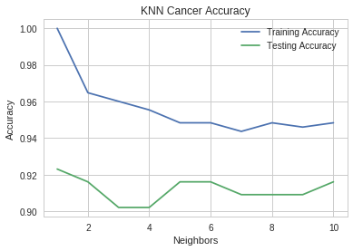
It looks like five neighbors would be what you'd want.

print("Minimum test accuracy (n=1): {:.2f}".format(min(testing_accuracies)))
print("Maximum test accuracy (n=5): {:.2f}".format(max(testing_accuracies)))
assert max(testing_accuracies == testing_accuracies[4])

Minimum test accuracy (n=1): 0.90
Maximum test accuracy (n=5): 0.92

The original paper that used this data-set got a cross-validation error-rate of 3%, but it sounds like they didn't split the data into training and testing sets (I'll have to re-read the paper to be sure).