Linear Models

1 Linear Regression

import matplotlib.pyplot as pyplot
import pandas
import seaborn
from sklearn.linear_model import (
    Lasso,
    LinearRegression,
    Ridge,
    )
from sklearn.datasets import load_boston
from sklearn.model_selection import train_test_split

%matplotlib inline
seaborn.set_style("whitegrid")

boston = load_boston()
print("Boston data-shape: {0}".format(boston.data.shape))

Boston data-shape: (506, 13)

X_train, X_test, y_train, y_test = train_test_split(boston.data, boston.target)

1.3 The Model

model = LinearRegression()
model.fit(X_train, y_train)

print("coefficients: {0}".format(model.coef_))
print("intercept: {0}".format(model.intercept_))

coefficients: [ -5.29188465e-02   3.27516047e-02   5.15495287e-02   1.96191849e+00
  -1.70355026e+01   4.26984342e+00  -4.66261395e-03  -1.24731581e+00
   2.40316945e-01  -1.12757320e-02  -9.67653044e-01   1.07129222e-02
  -4.58665079e-01]
intercept: 31.315219281412134

pollution_index = 4
names = ["Crime", "Large Lots", "Non-Retail Businesses",
         "Charles River adjacent", "Nitric Oxide", "Rooms", "Old Homes",
         "Distance to Employment", "Access to Highways", "Tax Rate",
         "Pupil-Teacher Ratio", "Blacks", "Lower Status"]
pandas.Series(model.coef_, index=names)

Crime                     -0.052919
Large Lots                 0.032752
Non-Retail Businesses      0.051550
Charles River adjacent     1.961918
Nitric Oxide             -17.035503
Rooms                      4.269843
Old Homes                 -0.004663
Distance to Employment    -1.247316
Access to Highways         0.240317
Tax Rate                  -0.011276
Pupil-Teacher Ratio       -0.967653
Blacks                     0.010713
Lower Status              -0.458665
dtype: float64

The price of homes in Boston is negatively correlated with Crime, Nitric Oxide (pollution), Distance to employment centes, Tax Rate, Pupil:Teacher ratio and the Lower status of the residents, with pollution being the overall largest factor (positive or negative). The most positive factors were the number of rooms the house had and whether the house was adjacent to the Charles River.

print("Training r2: {:.2f}".format(model.score(X_train, y_train)))
print("Testing r2: {0:.2f}".format(model.score(X_test, y_test)))

Training r2: 0.74
Testing r2: 0.73

The training and testing scores were oddly close, suggesting that this model generalizes well.

training = pandas.DataFrame(X_train, columns=names)

seaborn.pairplot(training)

2 Ridge Regression

This model uses L2 regression to reduce the size of the coefficients.

ridge = Ridge()
ridge.fit(X_train, y_train)

print("Training r2: {0:.2f}".format(ridge.score(X_train, y_train)))
print("Testing r2: {:.2f}".format(ridge.score(X_test, y_test)))

Training r2: 0.74
Testing r2: 0.72

This time the testing did a little worse than without ridge regression.

pandas.Series(ridge.coef_, index=names)

Crime                    -0.048337
Large Lots                0.032897
Non-Retail Businesses     0.016831
Charles River adjacent    1.789245
Nitric Oxide             -8.860668
Rooms                     4.270665
Old Homes                -0.011137
Distance to Employment   -1.125192
Access to Highways        0.224993
Tax Rate                 -0.012211
Pupil-Teacher Ratio      -0.891977
Blacks                    0.010977
Lower Status             -0.471429
dtype: float64

Once again pollution and the number of rooms a home had were the biggest influence on the price of the home.

3 Lasso Regression

This model uses L1 regression to remove the variables that don't influenc the outcome.

lasso = Lasso()
lasso.fit(X_train, y_train)

print("Training r2: {0:.2f}".format(lasso.score(X_train, y_train)))
print("Testing r2: {0:.2f}".format(lasso.score(X_test, y_test)))

Training r2: 0.67
Testing r2: 0.64

The Lasso did worse than the Ridge and ordinary-least-squares models did.

coefficients = pandas.Series(lasso.coef_, index=names)
coefficients[coefficients==0]

Non-Retail Businesses    -0.0
Charles River adjacent    0.0
Nitric Oxide             -0.0
dtype: float64

The Lasso removed Non-Retail Businesses, Charles River adjacency, and pollution, even though the other models decided that pollution was the most important factor.

We can try and do better by using a less aggressive alpha value.

lasso = Lasso(alpha=0.01)
lasso.fit(X_train, y_train)
print("Training r2: {0:.2f}".format(lasso.score(X_train, y_train)))
print("Testing r2: {0:.2f}".format(lasso.score(X_test, y_test)))
coefficients = pandas.Series(lasso.coef_, index=names)
print(coefficients[coefficients==0])

Training r2: 0.74
Testing r2: 0.73
Series([], dtype: float64)

Tuning the alpha can make it perform slightly better than the Ridge regression, but in this case making it aggressive enough to get rid of a column ("Nitric Oxide") makes it perform slightl worse than Ride regression.

training = pandas.DataFrame(X_train, columns=names)
training["price"] = y_train
seaborn.regplot(x="Nitric Oxide", y="price", data=training)
pyplot.xlabel("Nitric Oxide")
pyplot.ylabel("House Price")
pyplot.title("Pollution vs House Price")

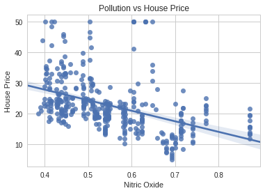
It appears that there is a linear relationship (although there are what appears to be some outliers).