Dog and Cat Breed Classification (What's Your Pet?)
Table of Contents
Departure
This is lesson one from the fastai course Practical Deep Learning for Coders, v3, which I assume is the third version of the course, and not a reference to a Japanese television show. It uses the fastai V1 library which uses Pytorch 1.0 but is an opinionated framework that bundles some sensible defaults so you don't have to spend as much time building the networks.
The goal is to train a neural network to identify the breeds of cats and dogs based of photos of them. It uses the Oxford-IIT Pet Dataset which was created by researchers at Oxford University's Visual Geometry Group.
Imports
Python
Other than the re none of the python imports were part of the original lesson. I'm importing gc to do garbage collection because the lesson starts with a smaller network and then changes to a larger one which caused my machine to run out of memory on the GPU. The rest of the imports are for settings and setup.
from argparse import Namespace
from functools import partial
from pathlib import Path
import gc
import os
import re
PyPi
fastai recommends using * to import everything, but I'd like to know where everything comes from and not import something that might conflict with my naming conventions so I'm going to (at least try to) import things individually. Luckily, unlike some projects (I'm looking at you, bokeh), their site has a search feature so you can look things up to see which module they come from.
I'll keep the fast.ai stuff separate to maybe make it easier to reference what comes from where.
from fastai.datasets import untar_data, URLs
from fastai.metrics import accuracy, error_rate
from fastai.train import ClassificationInterpretation
from fastai.vision.data import (
    get_image_files,
    imagenet_stats,
    ImageDataBunch)
from fastai.vision.learner import cnn_learner
from fastai.vision.models import resnet18, resnet34, resnet50
from fastai.vision.transform import get_transforms
And the rest…
from dotenv import load_dotenv
from ipyexperiments import IPyExperimentsPytorch
from tabulate import tabulate
import holoviews
import matplotlib.pyplot as pyplot
import numpy
import pandas
import seaborn
import torch
My Stuff
This is just some convenience stuff wrapped around other people's code (my lite-version of opinionated code).
from graeae.tables import CountPercentage
from graeae.timers import Timer
from graeae.visualization import EmbedHoloview
Some Setup
Some Constants
There's a lot of values scattered all over the place and I just wanted one place to keep track of them and maybe change them if needed.
Net = Namespace(
    random_seed=2,
    batch_size=64,
    low_memory_batch_size=16,
)
The Random Seed
To make this reproducible I'll set the random seed in numpy.
numpy.random.seed(Net.random_seed)
The Path
This loads where I put the image data-set.
load_dotenv(".env", override=True)
DATA_PATH = Path(os.environ.get("OXFORD_PET_DATASET")).expanduser()
Plotting
Although I'd prefer to plot things in HoloViews/bokeh, some of their stuff is too tightly bundled to make it easy (and the image plots maybe don't need to be interactive) so this sets up some formatting for the matplotlib plots.
Matplotlib
get_ipython().run_line_magic('matplotlib', 'inline')
get_ipython().run_line_magic('config', "InlineBackend.figure_format = 'retina'")
seaborn.set(style="whitegrid",
            rc={"axes.grid": False,
                "font.family": ["sans-serif"],
                "font.sans-serif": ["Open Sans", "Latin Modern Sans", "Lato"],
                "figure.figsize": (8, 6)},
            font_scale=1)
The Bokeh
This sets up some stuff for the javascript-based plotting.
holoviews.extension("bokeh")
SLUG = "dog-and-cat-breed-classification"
OUTPUT_FOLDER = Path("../../files/posts/fastai/")/SLUG
Embed = partial(EmbedHoloview, folder_path=OUTPUT_FOLDER)
This is where I'm going to put the settings for the javascript-based plotting.
Plot = Namespace(
    width = 1000,
    height = 800,
)
The Timer
This times how long things take so I can estimate how long it will take if I re-run cells. It also speaks a message so I can do something else and will know that the code is done running without having to watch the messages.
TIMER = Timer()
Tabulate
This is to format tables in the org-mode format (since I'm running this in emacs org-babel).
ORG_TABLE = partial(tabulate, headers="keys",
                    showindex=False,
                    tablefmt="orgtbl")
Initiation
Downloading the Data
As I mentioned before, the data will be the Oxford-IIIT Pet Dataset by O. M. Parkhi et al., 2012. In the dataset there are twelve breeds of cat and twenty-five breeds of dog. When the researchers performed their experiments in 2012 the best accuracy they got was 59.21 %.
The original lesson uses the untar_data function to download the data-set.
help(untar_data)
Help on function untar_data in module fastai.datasets:

untar_data(url: str, fname: Union[pathlib.Path, str] = None, dest: Union[pathlib.Path, str] = None, data=True, force_download=False) -> pathlib.Path
    Download `url` to `fname` if it doesn't exist, and un-tgz to folder `dest`.
This data set is 774 Megabytes and given my over-priced yet still incredibly slow CenturyLink speeds I found downloading it directly from the fastai datasets page a little more satisfactory, since the progress widget that runs during the download when untar_data downloads the dataset doesn't show up in emacs.
assert DATA_PATH.is_dir()
print(DATA_PATH)
/home/athena/data/datasets/images/oxford-iiit-pet
I didn't know it, but Paths have an ls method (so far as I could see this isn't in python's documentation) which I mention because I found out because it was in the original lesson. This is nice because, well, it's easy to remember, but the way I'm using it iterdir makes more sense.
for path in DATA_PATH.iterdir():
    print(f" - {path}")
- /home/athena/data/datasets/images/oxford-iiit-pet/images_backup
- /home/athena/data/datasets/images/oxford-iiit-pet/README.org
- /home/athena/data/datasets/images/oxford-iiit-pet/images
- /home/athena/data/datasets/images/oxford-iiit-pet/annotations
Here's another trick I didn't know about, but learned from the lesson - instead of using the joinpath method you can just use a forward-slash.
path_to_annotations = DATA_PATH/'annotations'
path_to_images = DATA_PATH/'images'
Looking At the Data
Getting the Labels
Here's where we peek at our data set. The dataset is set up so that the breeds are used in the names of the image files. fast.ai has a convenient classmethod named ImageDataBunch.from_name_re that will extract the labels from the filenames using a regular expression.
Before we get to that, though, we can take a look at some file names using get_image_files.
file_names = get_image_files(path_to_images)
for path in file_names[:5]:
    print(f" - {path.name}")
- Boxer_20.jpg
- Saint_Bernard_195.jpg
- Saint_Bernard_133.jpg
- English_Cocker_Spaniel_43.jpg
- Pug_51.jpg
So it looks like the format is <breed>_<index>.jpg. Later on we're going to use the labels when we inspect the model so next I'm going to make the standardize the file-name cases to be title-cased.
UNDERSCORE, SPACE = "_", " "
for path in file_names:
    name, extension = os.path.splitext(path.name)
    name = name.replace(UNDERSCORE, SPACE).title()
    file_name = (name + extension).replace(SPACE, UNDERSCORE)
    target = path.parent.joinpath(file_name)
    path.rename(target)

file_names = get_image_files(path_to_images)
for path in file_names[:2]:
    print(f" - {path.name}")
- Boxer_20.jpg
- Saint_Bernard_195.jpg
Now I'll construct the pattern to match the file-name.
is_not_a = "^"
end_of_line = "$"
one_or_more = "+"
digit = r"\d"
forward_slash = "/"
character_class = "[{}]"
group = "({})"

anything_but_a_slash = character_class.format(f"{is_not_a}{forward_slash}")

index = rf"{digit}{one_or_more}"
label = group.format(f'{anything_but_a_slash}{one_or_more}')
file_extension = ".jpg"

expression = rf'{forward_slash}{label}{UNDERSCORE}{index}{file_extension}{end_of_line}'
test = "/home/athena/data/datasets/images/oxford-iiit-pet/images/Saint_Bernard_195.jpg"
assert re.search(expression, test).groups()[0] == "Saint_Bernard"
The reason for the forward slash at the beginning of the expression is that we're passing in the entire path to each image, not just the name of the image.
Now on to the ImageDataBunch. Here's the arguments we need to pass in.
print(help(ImageDataBunch.from_name_re))
Help on method from_name_re in module fastai.vision.data:

from_name_re(path: Union[pathlib.Path, str], fnames: Collection[pathlib.Path], pat: str, valid_pct: float = 0.2, **kwargs) method of builtins.type instance
    Create from list of `fnames` in `path` with re expression `pat`.

None
Okay, so let's get the labels.
data = ImageDataBunch.from_name_re(path_to_images,
                                   file_names,
                                   expression,
                                   ds_tfms=get_transforms(),
                                   size=224,
                                   bs=Net.batch_size
                                  ).normalize(imagenet_stats)
One of the arguments we passed in (ds_tfms?) isn't particularly obviously named, unless you already know about applying transforms to images, but here's what we passed to it.
print(help(get_transforms))
Help on function get_transforms in module fastai.vision.transform:

get_transforms(do_flip:bool=True, flip_vert:bool=False, max_rotate:float=10.0, max_zoom:float=1.1, max_lighting:float=0.2, max_warp:float=0.2, p_affine:float=0.75, p_lighting:float=0.75, xtra_tfms:Union[Collection[fastai.vision.image.Transform], NoneType]=None) -> Collection[fastai.vision.image.Transform]
    Utility func to easily create a list of flip, rotate, `zoom`, warp, lighting transforms.

None
get_transforms adds random changes to the images to augment the datasets for our training.
We also added a call to normalize which sets the mean and standard deviation of the images to match those of the images used to train the model that we're going to use (ResNet).
Looking at Some of the Images
The show_batch method will plot some of the images in matplotlib. It retrieves them randomly so calling the method repeatedly will pull up different images. Unfortunately you can't pass in a figure or axes so it isn't easily configurable.
help(data.show_batch)
Help on method show_batch in module fastai.basic_data:

show_batch(rows:int=5, ds_type:fastai.basic_data.DatasetType=<DatasetType.Train: 1>, reverse:bool=False, **kwargs) -> None method of fastai.vision.data.ImageDataBunch instance
    Show a batch of data in `ds_type` on a few `rows`.
data.show_batch(rows=3, figsize=(7,6))
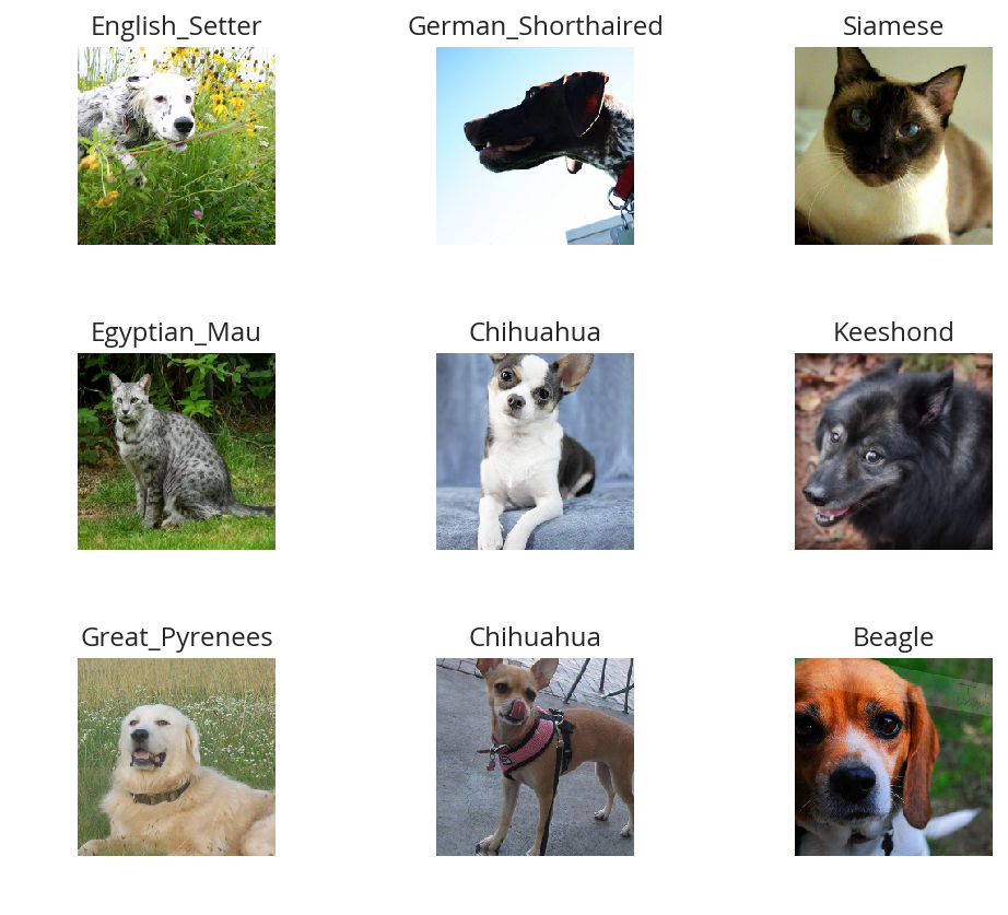
I'm guessing that the reason why so many images look "off" is because the of the data-transforms being added, and not that the photographers were horrible (or drunk). Why don't we look at the representation of the data bunch?
print(data)
ImageDataBunch;

Train: LabelList (5912 items)
x: ImageList
Image (3, 224, 224),Image (3, 224, 224),Image (3, 224, 224),Image (3, 224, 224),Image (3, 224, 224)
y: CategoryList
Boxer,Saint_Bernard,Saint_Bernard,Ragdoll,Birman
Path: /home/athena/data/datasets/images/oxford-iiit-pet/images;

Valid: LabelList (1478 items)
x: ImageList
Image (3, 224, 224),Image (3, 224, 224),Image (3, 224, 224),Image (3, 224, 224),Image (3, 224, 224)
y: CategoryList
Siamese,British_Shorthair,English_Cocker_Spaniel,Newfoundland,Russian_Blue
Path: /home/athena/data/datasets/images/oxford-iiit-pet/images;

Test: None
So it looks like the ImageDataBunch created a training and a validation set and each of the images has three channels and is 224 x 224 pixels.
Training: resnet34
Here's where we train the model, a convolutional neural network in the back with a fully-connected network at the end.
I'll use fast.ai's cnn_learner to load the data, pre-trained model (resnet34), and the metric to use when training (error_rate). If you look at the fast ai code they are importing the resnet34 model from pytorch's torchvision.
This next block sets up the IPyExperiments which will delete all the variables that were created after it was created when it is deleted. This is to free up memory because the resnet architecture takes up a lot of memory on the GPU.
experiment = IPyExperimentsPytorch()
Experiment started with the Pytorch backend
Device: ID 0, GeForce GTX 1060 6GB (6069 RAM)
Current state:
RAM: Used Free Total Util CPU: 2,375 58,710 64,336 MB 3.69% GPU: 916 5,153 6,069 MB 15.10%
・ RAM: △Consumed △Peaked Used Total | Exec time 0:00:00.000 ・ CPU: 0 0 2,375 MB | ・ GPU: 0 0 916 MB |
learn = cnn_learner(data, resnet34, metrics=error_rate)
・ RAM:  △Consumed    △Peaked    Used Total | Exec time 0:00:01.758
・ CPU:          0          0      2,551 MB |
・ GPU:        114          0      1,030 MB |
Downloading: "https://download.pytorch.org/models/resnet34-333f7ec4.pth" to /home/athena/.torch/models/resnet34-333f7ec4.pth
87306240it [00:26, 3321153.99it/s]
As you can see, it downloaded the stored model parameters from pytorch. This is because I've never downloaded this particular model before - if you run it again it shouldn't need to re-download it. Since this is a pytorch model we can look at it's represetantion to see the architecture of the network.
print(learn.model)
Sequential(
  (0): Sequential(
    (0): Conv2d(3, 64, kernel_size=(7, 7), stride=(2, 2), padding=(3, 3), bias=False)
    (1): BatchNorm2d(64, eps=1e-05, momentum=0.1, affine=True, track_running_stats=True)
    (2): ReLU(inplace)
    (3): MaxPool2d(kernel_size=3, stride=2, padding=1, dilation=1, ceil_mode=False)
    (4): Sequential(
      (0): BasicBlock(
        (conv1): Conv2d(64, 64, kernel_size=(3, 3), stride=(1, 1), padding=(1, 1), bias=False)
        (bn1): BatchNorm2d(64, eps=1e-05, momentum=0.1, affine=True, track_running_stats=True)
        (relu): ReLU(inplace)
        (conv2): Conv2d(64, 64, kernel_size=(3, 3), stride=(1, 1), padding=(1, 1), bias=False)
        (bn2): BatchNorm2d(64, eps=1e-05, momentum=0.1, affine=True, track_running_stats=True)
      )
      (1): BasicBlock(
        (conv1): Conv2d(64, 64, kernel_size=(3, 3), stride=(1, 1), padding=(1, 1), bias=False)
        (bn1): BatchNorm2d(64, eps=1e-05, momentum=0.1, affine=True, track_running_stats=True)
        (relu): ReLU(inplace)
        (conv2): Conv2d(64, 64, kernel_size=(3, 3), stride=(1, 1), padding=(1, 1), bias=False)
        (bn2): BatchNorm2d(64, eps=1e-05, momentum=0.1, affine=True, track_running_stats=True)
      )
      (2): BasicBlock(
        (conv1): Conv2d(64, 64, kernel_size=(3, 3), stride=(1, 1), padding=(1, 1), bias=False)
        (bn1): BatchNorm2d(64, eps=1e-05, momentum=0.1, affine=True, track_running_stats=True)
        (relu): ReLU(inplace)
        (conv2): Conv2d(64, 64, kernel_size=(3, 3), stride=(1, 1), padding=(1, 1), bias=False)
        (bn2): BatchNorm2d(64, eps=1e-05, momentum=0.1, affine=True, track_running_stats=True)
      )
    )
    (5): Sequential(
      (0): BasicBlock(
        (conv1): Conv2d(64, 128, kernel_size=(3, 3), stride=(2, 2), padding=(1, 1), bias=False)
        (bn1): BatchNorm2d(128, eps=1e-05, momentum=0.1, affine=True, track_running_stats=True)
        (relu): ReLU(inplace)
        (conv2): Conv2d(128, 128, kernel_size=(3, 3), stride=(1, 1), padding=(1, 1), bias=False)
        (bn2): BatchNorm2d(128, eps=1e-05, momentum=0.1, affine=True, track_running_stats=True)
        (downsample): Sequential(
          (0): Conv2d(64, 128, kernel_size=(1, 1), stride=(2, 2), bias=False)
          (1): BatchNorm2d(128, eps=1e-05, momentum=0.1, affine=True, track_running_stats=True)
        )
      )
      (1): BasicBlock(
        (conv1): Conv2d(128, 128, kernel_size=(3, 3), stride=(1, 1), padding=(1, 1), bias=False)
        (bn1): BatchNorm2d(128, eps=1e-05, momentum=0.1, affine=True, track_running_stats=True)
        (relu): ReLU(inplace)
        (conv2): Conv2d(128, 128, kernel_size=(3, 3), stride=(1, 1), padding=(1, 1), bias=False)
        (bn2): BatchNorm2d(128, eps=1e-05, momentum=0.1, affine=True, track_running_stats=True)
      )
      (2): BasicBlock(
        (conv1): Conv2d(128, 128, kernel_size=(3, 3), stride=(1, 1), padding=(1, 1), bias=False)
        (bn1): BatchNorm2d(128, eps=1e-05, momentum=0.1, affine=True, track_running_stats=True)
        (relu): ReLU(inplace)
        (conv2): Conv2d(128, 128, kernel_size=(3, 3), stride=(1, 1), padding=(1, 1), bias=False)
        (bn2): BatchNorm2d(128, eps=1e-05, momentum=0.1, affine=True, track_running_stats=True)
      )
      (3): BasicBlock(
        (conv1): Conv2d(128, 128, kernel_size=(3, 3), stride=(1, 1), padding=(1, 1), bias=False)
        (bn1): BatchNorm2d(128, eps=1e-05, momentum=0.1, affine=True, track_running_stats=True)
        (relu): ReLU(inplace)
        (conv2): Conv2d(128, 128, kernel_size=(3, 3), stride=(1, 1), padding=(1, 1), bias=False)
        (bn2): BatchNorm2d(128, eps=1e-05, momentum=0.1, affine=True, track_running_stats=True)
      )
    )
    (6): Sequential(
      (0): BasicBlock(
        (conv1): Conv2d(128, 256, kernel_size=(3, 3), stride=(2, 2), padding=(1, 1), bias=False)
        (bn1): BatchNorm2d(256, eps=1e-05, momentum=0.1, affine=True, track_running_stats=True)
        (relu): ReLU(inplace)
        (conv2): Conv2d(256, 256, kernel_size=(3, 3), stride=(1, 1), padding=(1, 1), bias=False)
        (bn2): BatchNorm2d(256, eps=1e-05, momentum=0.1, affine=True, track_running_stats=True)
        (downsample): Sequential(
          (0): Conv2d(128, 256, kernel_size=(1, 1), stride=(2, 2), bias=False)
          (1): BatchNorm2d(256, eps=1e-05, momentum=0.1, affine=True, track_running_stats=True)
        )
      )
      (1): BasicBlock(
        (conv1): Conv2d(256, 256, kernel_size=(3, 3), stride=(1, 1), padding=(1, 1), bias=False)
        (bn1): BatchNorm2d(256, eps=1e-05, momentum=0.1, affine=True, track_running_stats=True)
        (relu): ReLU(inplace)
        (conv2): Conv2d(256, 256, kernel_size=(3, 3), stride=(1, 1), padding=(1, 1), bias=False)
        (bn2): BatchNorm2d(256, eps=1e-05, momentum=0.1, affine=True, track_running_stats=True)
      )
      (2): BasicBlock(
        (conv1): Conv2d(256, 256, kernel_size=(3, 3), stride=(1, 1), padding=(1, 1), bias=False)
        (bn1): BatchNorm2d(256, eps=1e-05, momentum=0.1, affine=True, track_running_stats=True)
        (relu): ReLU(inplace)
        (conv2): Conv2d(256, 256, kernel_size=(3, 3), stride=(1, 1), padding=(1, 1), bias=False)
        (bn2): BatchNorm2d(256, eps=1e-05, momentum=0.1, affine=True, track_running_stats=True)
      )
      (3): BasicBlock(
        (conv1): Conv2d(256, 256, kernel_size=(3, 3), stride=(1, 1), padding=(1, 1), bias=False)
        (bn1): BatchNorm2d(256, eps=1e-05, momentum=0.1, affine=True, track_running_stats=True)
        (relu): ReLU(inplace)
        (conv2): Conv2d(256, 256, kernel_size=(3, 3), stride=(1, 1), padding=(1, 1), bias=False)
        (bn2): BatchNorm2d(256, eps=1e-05, momentum=0.1, affine=True, track_running_stats=True)
      )
      (4): BasicBlock(
        (conv1): Conv2d(256, 256, kernel_size=(3, 3), stride=(1, 1), padding=(1, 1), bias=False)
        (bn1): BatchNorm2d(256, eps=1e-05, momentum=0.1, affine=True, track_running_stats=True)
        (relu): ReLU(inplace)
        (conv2): Conv2d(256, 256, kernel_size=(3, 3), stride=(1, 1), padding=(1, 1), bias=False)
        (bn2): BatchNorm2d(256, eps=1e-05, momentum=0.1, affine=True, track_running_stats=True)
      )
      (5): BasicBlock(
        (conv1): Conv2d(256, 256, kernel_size=(3, 3), stride=(1, 1), padding=(1, 1), bias=False)
        (bn1): BatchNorm2d(256, eps=1e-05, momentum=0.1, affine=True, track_running_stats=True)
        (relu): ReLU(inplace)
        (conv2): Conv2d(256, 256, kernel_size=(3, 3), stride=(1, 1), padding=(1, 1), bias=False)
        (bn2): BatchNorm2d(256, eps=1e-05, momentum=0.1, affine=True, track_running_stats=True)
      )
    )
    (7): Sequential(
      (0): BasicBlock(
        (conv1): Conv2d(256, 512, kernel_size=(3, 3), stride=(2, 2), padding=(1, 1), bias=False)
        (bn1): BatchNorm2d(512, eps=1e-05, momentum=0.1, affine=True, track_running_stats=True)
        (relu): ReLU(inplace)
        (conv2): Conv2d(512, 512, kernel_size=(3, 3), stride=(1, 1), padding=(1, 1), bias=False)
        (bn2): BatchNorm2d(512, eps=1e-05, momentum=0.1, affine=True, track_running_stats=True)
        (downsample): Sequential(
          (0): Conv2d(256, 512, kernel_size=(1, 1), stride=(2, 2), bias=False)
          (1): BatchNorm2d(512, eps=1e-05, momentum=0.1, affine=True, track_running_stats=True)
        )
      )
      (1): BasicBlock(
        (conv1): Conv2d(512, 512, kernel_size=(3, 3), stride=(1, 1), padding=(1, 1), bias=False)
        (bn1): BatchNorm2d(512, eps=1e-05, momentum=0.1, affine=True, track_running_stats=True)
        (relu): ReLU(inplace)
        (conv2): Conv2d(512, 512, kernel_size=(3, 3), stride=(1, 1), padding=(1, 1), bias=False)
        (bn2): BatchNorm2d(512, eps=1e-05, momentum=0.1, affine=True, track_running_stats=True)
      )
      (2): BasicBlock(
        (conv1): Conv2d(512, 512, kernel_size=(3, 3), stride=(1, 1), padding=(1, 1), bias=False)
        (bn1): BatchNorm2d(512, eps=1e-05, momentum=0.1, affine=True, track_running_stats=True)
        (relu): ReLU(inplace)
        (conv2): Conv2d(512, 512, kernel_size=(3, 3), stride=(1, 1), padding=(1, 1), bias=False)
        (bn2): BatchNorm2d(512, eps=1e-05, momentum=0.1, affine=True, track_running_stats=True)
      )
    )
  )
  (1): Sequential(
    (0): AdaptiveConcatPool2d(
      (ap): AdaptiveAvgPool2d(output_size=1)
      (mp): AdaptiveMaxPool2d(output_size=1)
    )
    (1): Flatten()
    (2): BatchNorm1d(1024, eps=1e-05, momentum=0.1, affine=True, track_running_stats=True)
    (3): Dropout(p=0.25)
    (4): Linear(in_features=1024, out_features=512, bias=True)
    (5): ReLU(inplace)
    (6): BatchNorm1d(512, eps=1e-05, momentum=0.1, affine=True, track_running_stats=True)
    (7): Dropout(p=0.5)
    (8): Linear(in_features=512, out_features=37, bias=True)
  )
)
That's a pretty big network, but the main thing to notice is the last layer, which has 37 out_features which corresponds to the number of breeds we have in our data-set. If you were working directly with pytorch you'd have to remove the last layer and add it back yourself, but fast.ai has done this for us.
Now we need to train it using the fit_one_cycle method. At first I thought 'one cycle' meant just one pass through the batches but according to the documentation, this is a reference to a training method called the 1Cycle Policy proposed by Leslie N. Smith that changes the hyperparameters to make the model train faster.
TIMER.mesasge = "Finished fitting the ResNet 34 Model."
with TIMER:
    learn.fit_one_cycle(4)
Started: 2019-04-21 18:18:45.894630
Ended: 2019-04-21 18:22:09.988508
Elapsed: 0:03:24.093878
・ RAM:  △Consumed    △Peaked    Used Total | Exec time 0:03:24.095
・ CPU:          0          0      2,999 MB |
・ GPU:        151      3,322      1,182 MB |
Depending on how busy the computer is this takes two to three minutes when I run it. Next let's store the parameters for the trained model to disk.
learn.save('stage-1')
・ RAM:  △Consumed    △Peaked    Used Total | Exec time 0:00:00.145
・ CPU:          0          0      3,000 MB |
・ GPU:         -1          0      1,181 MB |
Results
Let's look at how the model did. If I was running this in a jupyter notebook there would be a table output of the accuracy, but I'm not, and I can't find any documentation on how to get that myself, so, tough luck, then. We can look at some things after the fact, though - the ClassificationInterpretation class contains methods to help look at how the model did.
interpreter = ClassificationInterpretation.from_learner(learn)
The top_losses method returns a tuple of the highest losses along with the indices of the data that gave those losses. By default it actually gives all the losses sorted from largest to smallest, but you could pass in an integer to limit how much it returns.
losses, indexes = interpreter.top_losses()
print(losses)
print(indexes)
assert len(data.valid_ds)==len(losses)==len(indexes)
tensor([7.1777e+00, 6.8882e+00, 5.8577e+00,  ..., 3.8147e-06, 3.8147e-06,
        1.9073e-06])
tensor([1298, 1418,  166,  ...,  735,  404,  291])
・ RAM:  △Consumed    △Peaked    Used Total | Exec time 0:00:00.002
・ CPU:          0          0      3,000 MB |
・ GPU:          0          0      1,181 MB |
plot = holoviews.Distribution(losses).opts(title="Loss Distribution",
                                           xlabel="Loss",
                                           width=Plot.width,
                                           height=Plot.height)
Embed(plot=plot, file_name="loss_distribution")()
Although it looks like there are negative losses, that's just the way the distribution works out, it looks like most of the losses are around zero.
print(losses.max())
print(losses.min())
tensor(7.1777)
tensor(1.9073e-06)
・ RAM:  △Consumed    △Peaked    Used Total | Exec time 0:00:00.001
・ CPU:          0          0      3,000 MB |
・ GPU:          7          0      1,188 MB |
Here's a count of the losses when they are broken up into ten bins.
bins = pandas.cut(losses.tolist(), bins=10).value_counts().reset_index()
total = bins[0].sum()
percentage = 100 * bins[0]/total
bins["percent"] = percentage
print(ORG_TABLE(bins, headers="Range Count Percent(%)".split()))
| Range | Count | Percent(%) |
|---|---|---|
| (-0.00718, 0.718] | 1349 | 91.272 |
| (0.718, 1.436] | 61 | 4.1272 |
| (1.436, 2.153] | 31 | 2.09743 |
| (2.153, 2.871] | 14 | 0.947226 |
| (2.871, 3.589] | 15 | 1.01488 |
| (3.589, 4.307] | 3 | 0.202977 |
| (4.307, 5.024] | 2 | 0.135318 |
| (5.024, 5.742] | 0 | 0 |
| (5.742, 6.46] | 1 | 0.067659 |
| (6.46, 7.178] | 2 | 0.135318 |
It's not entirely clear to me how to interpret the losses - what does a loss of seven mean, exactly? -0.00744? But, anyway, it looks like the vast majority are less than one.
Another thing we can do is plot the images that had the highest losses.
interpreter.plot_top_losses(9, figsize=(15,11))
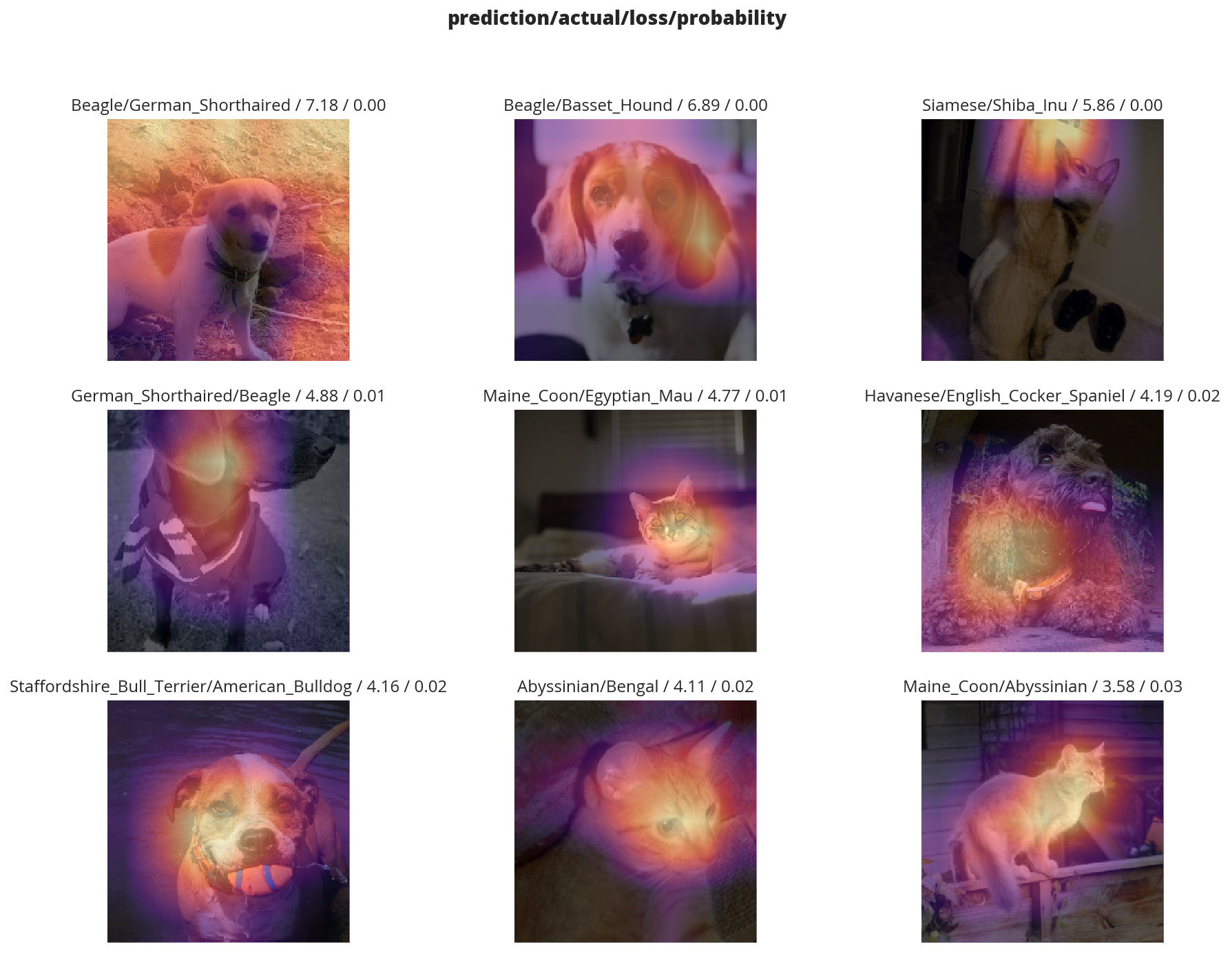
It looks like the ones that had the most loss had some kind of weird flare effect applied to the image. Now that we've used it, maybe we can see how we're supposed to call plot_top_losses.
print(help(interpreter.plot_top_losses))
Help on method _cl_int_plot_top_losses in module fastai.vision.learner:

_cl_int_plot_top_losses(k, largest=True, figsize=(12, 12), heatmap:bool=True, heatmap_thresh:int=16, return_fig:bool=None) -> Union[matplotlib.figure.Figure, NoneType] method of fastai.train.ClassificationInterpretation instance
    Show images in `top_losses` along with their prediction, actual, loss, and probability of actual class.

None
Note: in the original notebook they were using a function called doc, which tries to open another window and will thus hang when run in emacs. They really want you to use jupyter.
Next let's look at the confusion matrix.
interpreter.plot_confusion_matrix(figsize=(12,12), dpi=60)
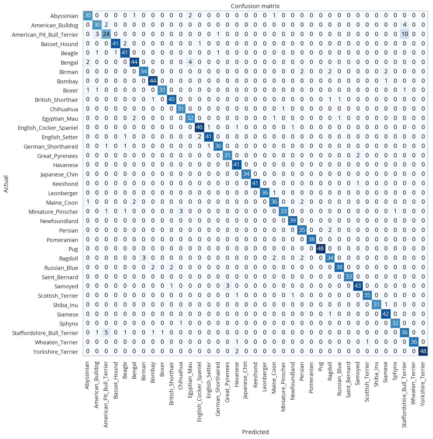
One way to interpret this is to look at the x-axis (the actual breed) and sweep vertically up to see the counts for the y-axis (what our model predicted it was). The diagonal cells from the top left to the bottom right is where the predicted matched the actual. In this case, the fact that almost all the counts are in the diagonal means our model did pretty well at predicting the breeds in the images.
If you compare the images with the worst losses to the confusion matrix you'll notice that they don't seem to correlate with the worst performances overall - the worst losses were one-offs, probably due to the flare effect. The most confused was the Ragdoll being confused for a Birman, but, as noted in the lecture, distinguishing them is hard for people too.
Here's the breeds that were the hardest for the model to predict.
print(ORG_TABLE(interpreter.most_confused(min_val=3),
                headers="Actual Predicted Count".split()))
| Actual | Predicted | Count |
|---|---|---|
| American_Pit_Bull_Terrier | Staffordshire_Bull_Terrier | 10 |
| Staffordshire_Bull_Terrier | American_Pit_Bull_Terrier | 5 |
| American_Bulldog | Staffordshire_Bull_Terrier | 4 |
| Bengal | Egyptian_Mau | 4 |
| American_Pit_Bull_Terrier | American_Bulldog | 3 |
| Miniature_Pinscher | Chihuahua | 3 |
| Ragdoll | Birman | 3 |
| Samoyed | Great_Pyrenees | 3 |
It doesn't look too bad, actually, other that the first few entries, maybe.
Unfreezing, fine-tuning, and learning rates
So, this is what we get with a straight off-the-shelf setup from fast.ai, but we want more, don't we? Let's unfreeze the model (allow the entire model's weights to be trained) and train some more.
learn.unfreeze()
Since we are using a pre-trained model we normally freeze all but the last layer to do transfer learning, by unfreezing the model we'll train all the layers to our dataset.
TIMER.message = "Finished training the unfrozen model."
with TIMER:
    learn.fit_one_cycle(1)
Started: 2019-04-21 18:29:47.149628
Ended: 2019-04-21 18:30:28.689325
Elapsed: 0:00:41.539697
・ RAM:  △Consumed    △Peaked    Used Total | Exec time 0:00:41.541
・ CPU:          0          0      3,010 MB |
・ GPU:        694      1,923      1,883 MB |
Now we save the parameters to disk again.
learn.save('stage-1');
Now we're going to use the lr_find method to find the best learning rate.
TIMER.message = "Finished finding the best learning rate."
with TIMER:
    learn.lr_find()
Started: 2019-04-21 18:31:02.961941
LR Finder is complete, type {learner_name}.recorder.plot() to see the graph.
Ended: 2019-04-21 18:31:29.892324
Elapsed: 0:00:26.930383
・ RAM:  △Consumed    △Peaked    Used Total | Exec time 0:00:26.931
・ CPU:          0          0      3,010 MB |
・ GPU:        339      1,646      2,218 MB |
learn.recorder.plot()
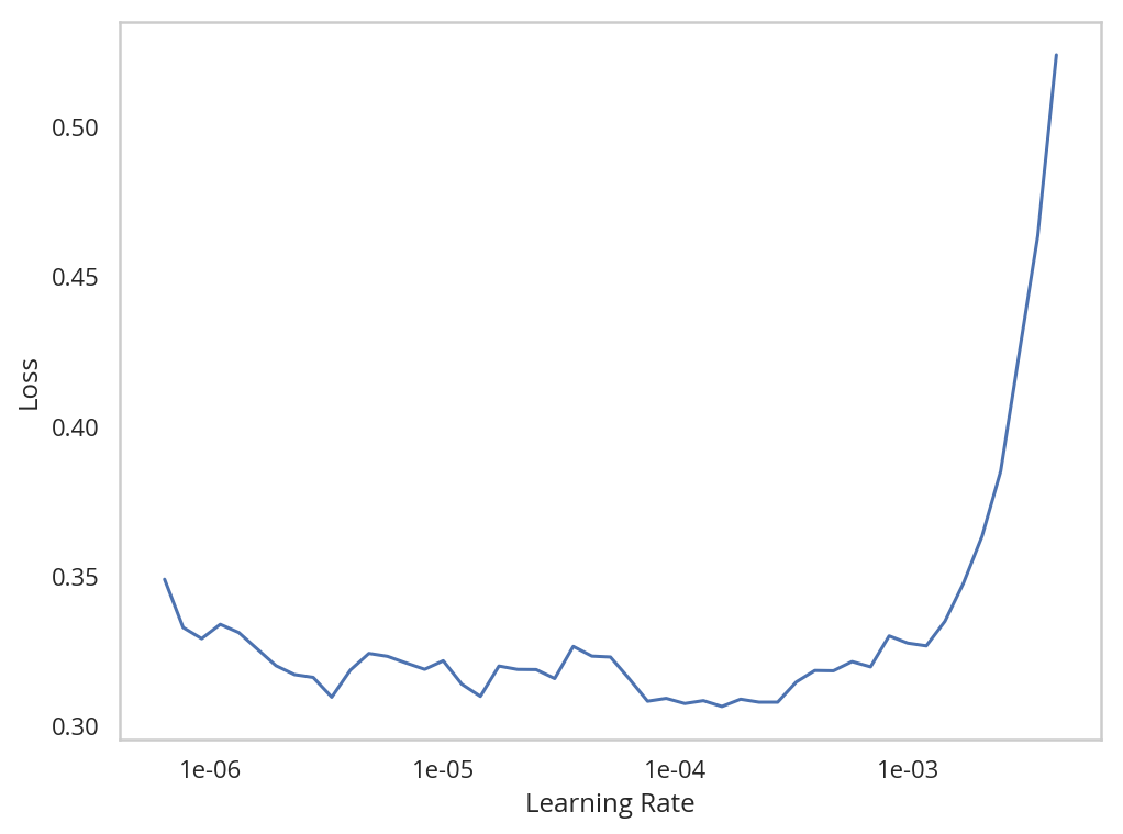
So, it's kind of hard to see the exact number, but you can see that somewhere around a learning rate of 0.0001 we get a good loss and then after that the loss starts to go way up.
So next we're going to re-train it using an interval that hopefully gives us the best loss.
learn.unfreeze()
with TIMER:
    print(learn.fit_one_cycle(2, max_lr=slice(1e-6,1e-4)))
Started: 2019-04-21 18:34:11.748741
None
Ended: 2019-04-21 18:35:34.827655
Elapsed: 0:01:23.078914
・ RAM:  △Consumed    △Peaked    Used Total | Exec time 0:01:23.083
・ CPU:          0          0      3,011 MB |
・ GPU:          9      1,634      2,231 MB |
Now the experiment is over so let's free up some memory.
del experiment
・ RAM: △Consumed △Peaked Used Total | Exec time 0:00:00.000 ・ CPU: 0 0 3,011 MB | ・ GPU: -17 0 2,214 MB |
IPyExperimentsPytorch: Finishing
Experiment finished in 00:20:22 (elapsed wallclock time)
Newly defined local variables:
Deleted: bins, codecs, indexes, interpreter, learn, losses, percentage, total
Circular ref objects gc collected during the experiment:
cleared 12 objects (only temporary leakage)
Experiment memory:
RAM: Consumed Reclaimed CPU: 636 0 MB ( 0.00%) GPU: 1,297 1,308 MB (100.82%)
Current state:
RAM: Used Free Total Util CPU: 3,011 57,984 64,336 MB 4.68% GPU: 906 5,163 6,069 MB 14.93%
Training: resnet50
Okay, so we trained the resnet34 model, and although I haven't figured out how to tell exactly how well it's doing, it seems to be doing pretty well. Now it's time to try the resnet50 model, which has pretty much the same architecture but more layers. This means it should do better, but it also takes up a lot more memory.
Even after deleting the old model I still run out of memory so I'm going to have to fall back to a smaller batch-size.
experiment = IPyExperimentsPytorch()
*** Experiment started with the Pytorch backend
Device: ID 0, GeForce GTX 1060 6GB (6069 RAM)


*** Current state:
RAM:    Used    Free   Total       Util
CPU:   3,011  57,984  64,336 MB   4.68%
GPU:     906   5,163   6,069 MB  14.93%


・ RAM:  △Consumed    △Peaked    Used Total | Exec time 0:00:00.000
・ CPU:          0          0      3,011 MB |
・ GPU:          0          0        906 MB |
data = ImageDataBunch.from_name_re(
    path_to_images,
    file_names,
    expression,
    ds_tfms=get_transforms(),
    size=299,
    bs=Net.low_memory_batch_size).normalize(imagenet_stats)
Now I'll re-build the learner with the new pre-trained model.
learn = cnn_learner(data, resnet50, metrics=error_rate)
learn.lr_find()
learn.recorder.plot()
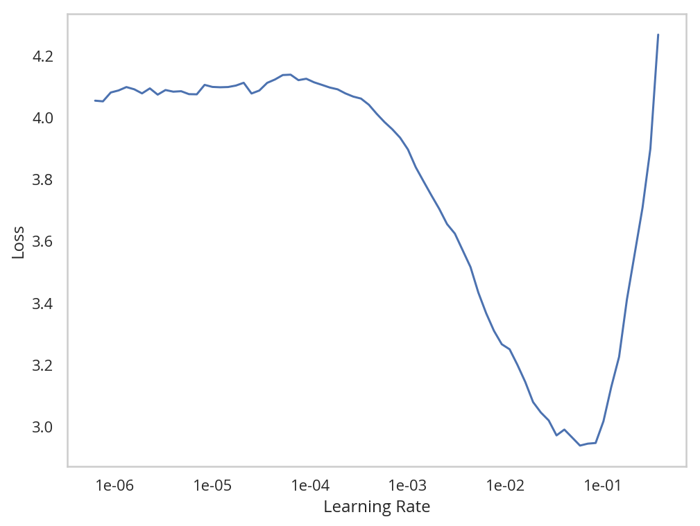
So with this learner we can see that there's a rapid drop in loss followed by a sudden spike in loss.
TIMER.message = "Done fitting resnet 50"
with TIMER:
    learn.fit_one_cycle(8)
Started: 2019-04-21 18:42:03.987300
Ended: 2019-04-21 18:57:43.628598
Elapsed: 0:15:39.641298
・ RAM:  △Consumed    △Peaked    Used Total | Exec time 0:15:39.643
・ CPU:          0          0      3,067 MB |
・ GPU:         17      4,474      1,117 MB |
Okay, so save the parameters again.
learn.save('stage-1-50')
Now we can try and unfreeze and re-train it.
TIMER.message = "Finished training resnet 50 with the optimal learning rate."
learn.unfreeze()
with TIMER:
    learn.fit_one_cycle(3, max_lr=slice(1e-6,1e-4))
Started: 2019-04-21 18:58:22.070603
Ended: 2019-04-21 19:06:24.471347
Elapsed: 0:08:02.400744
・ RAM:  △Consumed    △Peaked    Used Total | Exec time 0:08:02.406
・ CPU:          0          0      3,069 MB |
・ GPU:        259      4,586      1,376 MB |
with TIMER:
    metrics = learn.validate()
Started: 2019-04-21 19:08:37.971400
Ended: 2019-04-21 19:08:49.648814
Elapsed: 0:00:11.677414
・ RAM:  △Consumed    △Peaked    Used Total | Exec time 0:00:11.679
・ CPU:          0          0      3,069 MB |
・ GPU:         22        410      1,398 MB |
print(f"Error Rate: {metrics[0]:.2f}")
Error Rate: 0.15
Since it didn't improve let's go back to the previous model.
learn.load('stage-1-50');
with TIMER:
    metrics = learn.validate()
print(f"Error Rate: {metrics[0]:.2f}")
Started: 2019-04-21 19:09:19.655769
Ended: 2019-04-21 19:09:30.841289
Elapsed: 0:00:11.185520
Error Rate: 0.16
・ RAM:  △Consumed    △Peaked    Used Total | Exec time 0:00:16.011
・ CPU:          1          1      3,069 MB |
・ GPU:        308        612      1,706 MB |
Interpreting the Result
interpreter = ClassificationInterpretation.from_learner(learn)
The Most Confusing Breeds
print(ORG_TABLE(interpreter.most_confused(min_val=3),
                headers="Actual Predicted Count".split()))
| Actual | Predicted | Count |
|---|---|---|
| American_Pit_Bull_Terrier | Staffordshire_Bull_Terrier | 6 |
| Bengal | Egyptian_Mau | 5 |
| Ragdoll | Birman | 5 |
| Staffordshire_Bull_Terrier | American_Pit_Bull_Terrier | 5 |
| Bengal | Abyssinian | 3 |
It got fewer breeds with more than two wrong than the resnet34 model did, but both of them seem to have trouble telling an American Pit Bull Terrier from a Staffordshire Bull Terrier.
del experiment
・ RAM:  △Consumed    △Peaked    Used Total | Exec time 0:00:00.000
・ CPU:          0          0      3,070 MB |
・ GPU:          0          0      1,706 MB |
Other Data Formats
This is a look at other data sets.
MNIST
This is a set of handwritten digits. The originals are hosted on yann.lecun.com but the fast.ai datasets page has the images converted from the original IDX format to the PNG format.
experiment = IPyExperimentsPytorch()
*** Experiment started with the Pytorch backend
Device: ID 0, GeForce GTX 1060 6GB (6069 RAM)


*** Current state:
RAM:    Used    Free   Total       Util
CPU:   3,070  57,254  64,336 MB   4.77%
GPU:   1,706   4,363   6,069 MB  28.11%


・ RAM:  △Consumed    △Peaked    Used Total | Exec time 0:00:00.097
・ CPU:          0          0      3,070 MB |
・ GPU:          0          0      1,706 MB |
・ RAM:  △Consumed    △Peaked    Used Total | Exec time 0:00:00.043
・ CPU:          0          0      3,070 MB |
・ GPU:          0          0      1,706 MB |
mnist_path_original = Path(os.environ.get("MNIST")).expanduser()
assert mnist_path_original.is_dir()
print(mnist_path_original)
/home/athena/data/datasets/images/mnist_png
・ RAM:  △Consumed    △Peaked    Used Total | Exec time 0:00:00.001
・ CPU:          0          0      3,070 MB |
・ GPU:          0          0      1,706 MB |
・ RAM:  △Consumed    △Peaked    Used Total | Exec time 0:00:00.046
・ CPU:          0          0      3,070 MB |
・ GPU:          0          0      1,706 MB |
Now that we know it's there we can create a data bunch for it… Actually I tried it and found out that this is the wrong set (it throws an error for some reason), let's try it their way.
print(URLs.MNIST_SAMPLE)
mnist_path = untar_data(URLs.MNIST_SAMPLE)
print(mnist_path)
http://files.fast.ai/data/examples/mnist_sample
/home/athena/.fastai/data/mnist_sample
・ RAM:  △Consumed    △Peaked    Used Total | Exec time 0:00:00.309
・ CPU:          0          1      3,070 MB |
・ GPU:          0          0      1,706 MB |
・ RAM:  △Consumed    △Peaked    Used Total | Exec time 0:00:00.379
・ CPU:          0          0      3,070 MB |
・ GPU:          0          0      1,706 MB |
Let's look at the difference. Here's what I downloaded.
for path in mnist_path_original.iterdir():
    print(f" - {path}")
- /home/athena/data/datasets/images/mnist_png/testing
- /home/athena/data/datasets/images/mnist_png/README.org
- /home/athena/data/datasets/images/mnist_png/training
・ RAM: △Consumed △Peaked Used Total | Exec time 0:00:00.026 ・ CPU: 0 0 3,070 MB | ・ GPU: 0 0 1,706 MB | ・ RAM: △Consumed △Peaked Used Total | Exec time 0:00:00.071 ・ CPU: 0 0 3,070 MB | ・ GPU: 0 0 1,706 MB |
And here's what they downloaded.
for path in mnist_path.iterdir():
    print(f" - {path}")
- home/athena.fastai/data/mnist_sample/labels.csv
- home/athena.fastai/data/mnist_sample/train
- home/athena.fastai/data/mnist_sample/valid
- home/athena.fastai/data/mnist_sample/models
・ RAM: △Consumed △Peaked Used Total | Exec time 0:00:00.043 ・ CPU: 0 0 3,070 MB | ・ GPU: 0 0 1,706 MB | ・ RAM: △Consumed △Peaked Used Total | Exec time 0:00:00.090 ・ CPU: 0 0 3,070 MB | ・ GPU: 0 0 1,706 MB |
Maybe you need a labels.csv file… I guess that's the point of this being in the "other formats" section.
transforms = get_transforms(do_flip=False)
data = ImageDataBunch.from_folder(mnist_path, ds_tfms=transforms, size=26)
I don't know why the size is 26 in this case.
data.show_batch(rows=3, figsize=(5,5))
Now to fit the model. This uses a smaller version of the resnet (18 layers) and the accuracy metric.
with TIMER:
    learn = cnn_learner(data, resnet18, metrics=accuracy)
    learn.fit(2)
Started: 2019-04-21 19:15:13.568995
Ended: 2019-04-21 19:15:44.806330
Elapsed: 0:00:31.237335
・ RAM:  △Consumed    △Peaked    Used Total | Exec time 0:00:31.239
・ CPU:          0          0      3,075 MB |
・ GPU:         46      1,379      1,733 MB |
・ RAM:  △Consumed    △Peaked    Used Total | Exec time 0:00:31.297
・ CPU:          0          0      3,075 MB |
・ GPU:         46      1,379      1,733 MB |
So, since the labels are so important, maybe we should look at them.
labels = pandas.read_csv(mnist_path/'labels.csv')
print(ORG_TABLE(labels.iloc[:5]))
| name | label |
|---|---|
| train/3/7463.png | 0 |
| train/3/21102.png | 0 |
| train/3/31559.png | 0 |
| train/3/46882.png | 0 |
| train/3/26209.png | 0 |
Well, that's not realy revelatory.
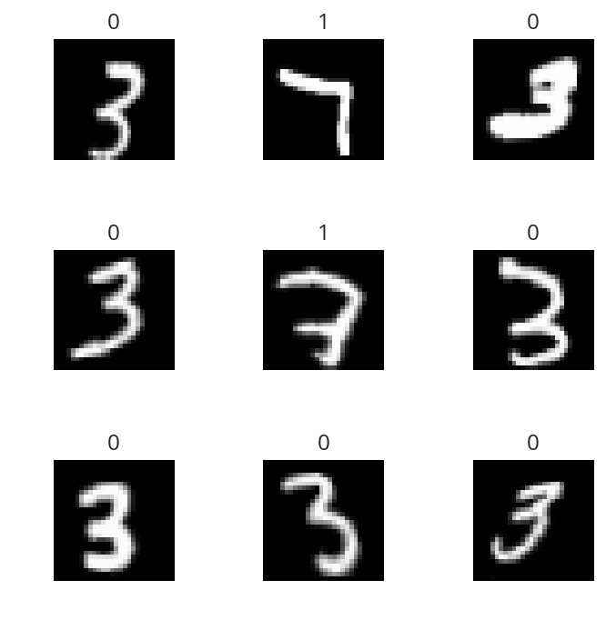
data = ImageDataBunch.from_csv(mnist_path, ds_tfms=transforms, size=28)
data.show_batch(rows=3, figsize=(5,5))
print(data.classes)
[0, 1]
・ RAM:  △Consumed    △Peaked    Used Total | Exec time 0:00:00.001
・ CPU:          0          0      3,080 MB |
・ GPU:          0          0      1,733 MB |
・ RAM:  △Consumed    △Peaked    Used Total | Exec time 0:00:00.047
・ CPU:          0          0      3,080 MB |
・ GPU:          0          0      1,733 MB |
So there are only two classes, presumably meaning that they are 3 and 7.
There's more examples of… something in the notebook, but they don't explain it so I'm just going to skip over the rest of it.
Return
This last bit just let's me run the whole notebook and get a message when it's over.
TIMER.message = "The Dog and cat breed classification buffer is done. Come check it out."
with TIMER:
    pass
Started: 2019-04-21 10:43:46.858157
Ended: 2019-04-21 10:43:46.858197
Elapsed: 0:00:00.000040