Compare and Learn
i#t+BEGIN_COMMENT .. title: Compare and Learn .. slug: compare-and-learn .. date: 2018-10-26 10:54:02 UTC-07:00 .. tags: grokking,gradient descent .. category: Grokking .. link: .. description: Introduction to Gradient Descent. .. type: text #+END_COMMENT
Table of Contents
Imports
From PyPi
from graphviz import Digraph
import matplotlib.pyplot as pyplot
import numpy
import pandas
import seaborn
Setup the plotting
%matplotlib inline
%config InlineBackend.figure_format='retina'
seaborn.set(style="whitegrid")
FIGURE_SIZE = (14, 12)
What is this about?
The three main steps in training a model are:
- Predict
- Compare
- Learn
Forward Propagation was about the Predict step - we fed some inputs to a network and it output its predictions. Now we're going to look an steps 2 and 3 - Compare and Learn, the steps where we figure out how to improve the weights in our network.
What's the next step after Predict?
As noted above, step 2 is Compare meaning compare our predictions with what we know to be the real answers (so this is supervised learning) and see how well (or bad) we did.
Okay, but then what?
After Compare we move on to the Learn step where we adjust the weights based on the errors we found in Compare. In this case we'll use Gradient Descent to find new weights for the network.
So, how do we find the error again?
There are many different ways to measure error, each with different positive and negative attributes, but in this case we're going to use Mean Squared Error. Here's an example with one measurement.
weight = 0.5
input_value = 0.5
expected = 0.8
actual = weight * input_value
# you implicitly divide by 1 to get the mean of the square
actual_error = (expected - actual)**2
expected_error = 0.3
assert abs(expected_error - actual_error) < 0.01
print("Error: {:.2f}".format(actual_error))
Error: 0.30
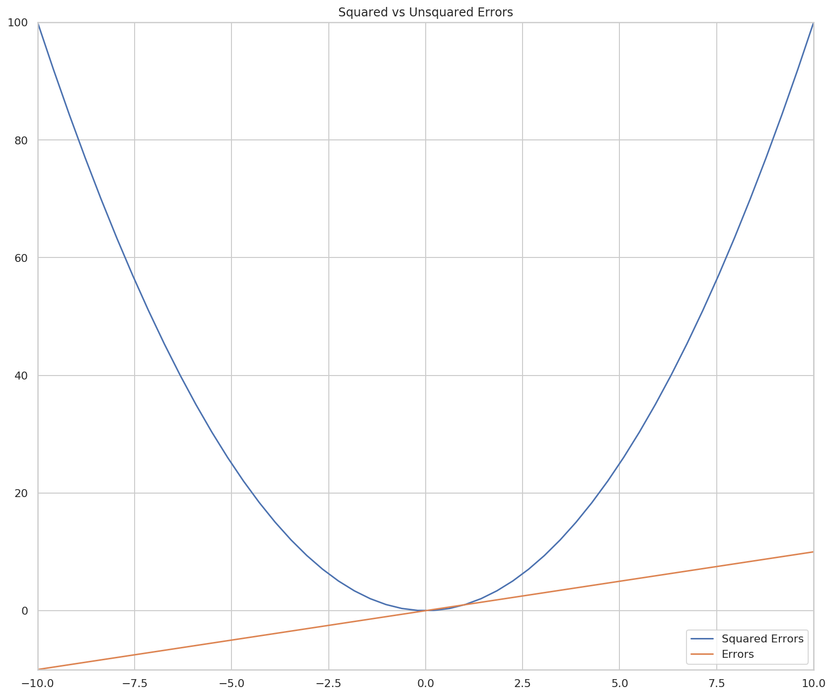
Two things to note about the consequences of squaring the error - one is that it's always positive which is useful because you might have both positive and negative errors which would tend to cancel each other out when you take the mean (the actual_error above is a mean with an implied count of 1), even though both positive and negative errors are wrong, the other consequence is that the greater the error, the larger it grows (it follows a parabola instead of a line).
figure, axe = pyplot.subplots(figsize=FIGURE_SIZE)
errors = numpy.linspace(-10, 10)
outputs = numpy.square(errors)
axe.set_xlim((-10, 10))
axe.set_ylim((-10, 100))
axe.set_title("Squared vs Unsquared Errors")
axe.plot(errors, outputs, label="Squared Errors" )
axe.plot(errors, errors, label="Errors")
legend = axe.legend()
So how do we learn?
One method is Hot-and-Cold Learning. With this method you move your weights a little and pick the one that improves the error-rate. This first example will go back to the one feature network that tries to predict if a team will win using the average number of toes they have.
graph = Digraph(comment="Toes", format="png")
graph.attr(rankdir="LR")
# input layer
graph.node("a", "Toes")

# output layer
graph.node("b", "Win")

# edge
graph.edge("a", "b", label="Weight")
graph.render("graphs/toes_model.dot")
graph

def toes_model(toes: int, weight: float=0.1) -> float:
    """Predicts if the team will win based on the number of toes

    Return:
     predction: probability of winning
    """
    return toes * weight
def print_error(predicted: float, actual: int, label: str="Toes Model",
                separator: str="\n") -> float:
    """Prints the (mean) squared error

    Args:

     predicted: what the model predicted
     actual: whether the team won or not
     label: something to identify the model
     separator: How to separate the output
    Returns:
     mse: the error
    """
    error = (actual - predicted)**2
    print(separator.join([label,
                          "Predicted: {:.2f}".format(predicted),
                          "Actual: {}".format(actual),
                          "MSE: {:.4f}".format(error)]))
    return error
toes = 8.5
actual = 1
predicted = toes_model(toes)
error_original = print_error(predicted, actual)
Toes Model
Predicted: 0.85
Actual: 1
MSE: 0.0225
So our model has a Mean Squared Error of around 0.02, how do we make it better with the Hot and Cold Method? By trying a larger and smaller weight and using the one that makes the error smaller.
weight_change = 0.01
weight = 0.1
knob_turned_up = toes_model(toes, weight + weight_change)
knob_turned_down = toes_model(toes, weight - weight_change)

error_up = print_error(knob_turned_up, actual, "Turned Up")
print()
error_down = print_error(knob_turned_down, actual, "Turned Down")
Turned Up
Predicted: 0.94
Actual: 1
MSE: 0.0042

Turned Down
Predicted: 0.77
Actual: 1
MSE: 0.0552
Looking at the error, it looks like making the weight higher improved the score, so we should adjust our weight upwards.
if error_original > error_up or error_original > error_down:
    change_direction = -1 if error_down < error_original else 1
    weight_updated = weight + change_direction * weight_change
    prediction = toes_model(toes, weight_updated)
    error_update = print_error(prediction, actual, "Updated Model")
    assert error_update < error_original
else:
    print("Model didn't improve.")
Updated Model
Predicted: 0.94
Actual: 1
MSE: 0.0042
So, this is what machine learning is really about, finding the parameters that give the best prediction. This is why it is often called a search problem - each of your parameters can have a variety of weights (infinite, actually) so what you are doing when you train your model is searching the space of weights to find the set that gives the best outcome for your metric. In this case we are looking to minimize our Mean Squared Error.
Training the Model
Rather than than trying to do the checks one at a time, we can run the Hot and Cold Learning in a loop to tune our model.
weight = 0.5
input_value = 0.5
actual = 0.8
weight_change = 0.001

prediction = toes_model(input_value, weight)
print_error(prediction, actual, "Step    1 Weight: {}".format(weight), "\t")
errors = []
weights = []
optimal_step = False
tolerance = 0.1**8
for step in range(1, 2001):
    prediction = toes_model(input_value, weight)
    error = (print_error(prediction, actual,
                         "Step {:4} Weight: {:.2f}".format(step, weight), "\t")
             if not step % 100 else (prediction - actual)**2)
    errors.append(error)
    if not optimal_step and error < tolerance:
        optimal_step = step - 1
    up_prediction = toes_model(input_value, weight + weight_change)
    down_prediction = toes_model(input_value, weight - weight_change)
    up_error = (up_prediction - actual)**2
    down_error = (down_prediction - actual)**2
    direction = -1 if down_error < up_error else 1
    weight += direction * weight_change
    weights.append(weight)

print("Optimum Reached at Step {}".format(optimal_step))
Step    1 Weight: 0.5   Predicted: 0.25 Actual: 0.8     MSE: 0.3025
Step  100 Weight: 0.60  Predicted: 0.30 Actual: 0.8     MSE: 0.2505
Step  200 Weight: 0.70  Predicted: 0.35 Actual: 0.8     MSE: 0.2030
Step  300 Weight: 0.80  Predicted: 0.40 Actual: 0.8     MSE: 0.1604
Step  400 Weight: 0.90  Predicted: 0.45 Actual: 0.8     MSE: 0.1229
Step  500 Weight: 1.00  Predicted: 0.50 Actual: 0.8     MSE: 0.0903
Step  600 Weight: 1.10  Predicted: 0.55 Actual: 0.8     MSE: 0.0628
Step  700 Weight: 1.20  Predicted: 0.60 Actual: 0.8     MSE: 0.0402
Step  800 Weight: 1.30  Predicted: 0.65 Actual: 0.8     MSE: 0.0227
Step  900 Weight: 1.40  Predicted: 0.70 Actual: 0.8     MSE: 0.0101
Step 1000 Weight: 1.50  Predicted: 0.75 Actual: 0.8     MSE: 0.0026
Step 1100 Weight: 1.60  Predicted: 0.80 Actual: 0.8     MSE: 0.0000
Step 1200 Weight: 1.60  Predicted: 0.80 Actual: 0.8     MSE: 0.0000
Step 1300 Weight: 1.60  Predicted: 0.80 Actual: 0.8     MSE: 0.0000
Step 1400 Weight: 1.60  Predicted: 0.80 Actual: 0.8     MSE: 0.0000
Step 1500 Weight: 1.60  Predicted: 0.80 Actual: 0.8     MSE: 0.0000
Step 1600 Weight: 1.60  Predicted: 0.80 Actual: 0.8     MSE: 0.0000
Step 1700 Weight: 1.60  Predicted: 0.80 Actual: 0.8     MSE: 0.0000
Step 1800 Weight: 1.60  Predicted: 0.80 Actual: 0.8     MSE: 0.0000
Step 1900 Weight: 1.60  Predicted: 0.80 Actual: 0.8     MSE: 0.0000
Step 2000 Weight: 1.60  Predicted: 0.80 Actual: 0.8     MSE: 0.0000
Optimum Reached at Step 1100
figure, axe = pyplot.subplots(figsize=FIGURE_SIZE)
axe.set_title("Hot and Cold Mean Squared Error")
axe.set_xlabel("Training Repetition")
axe.set_ylabel("MSE")
lines = axe.plot(range(len(errors)), errors)
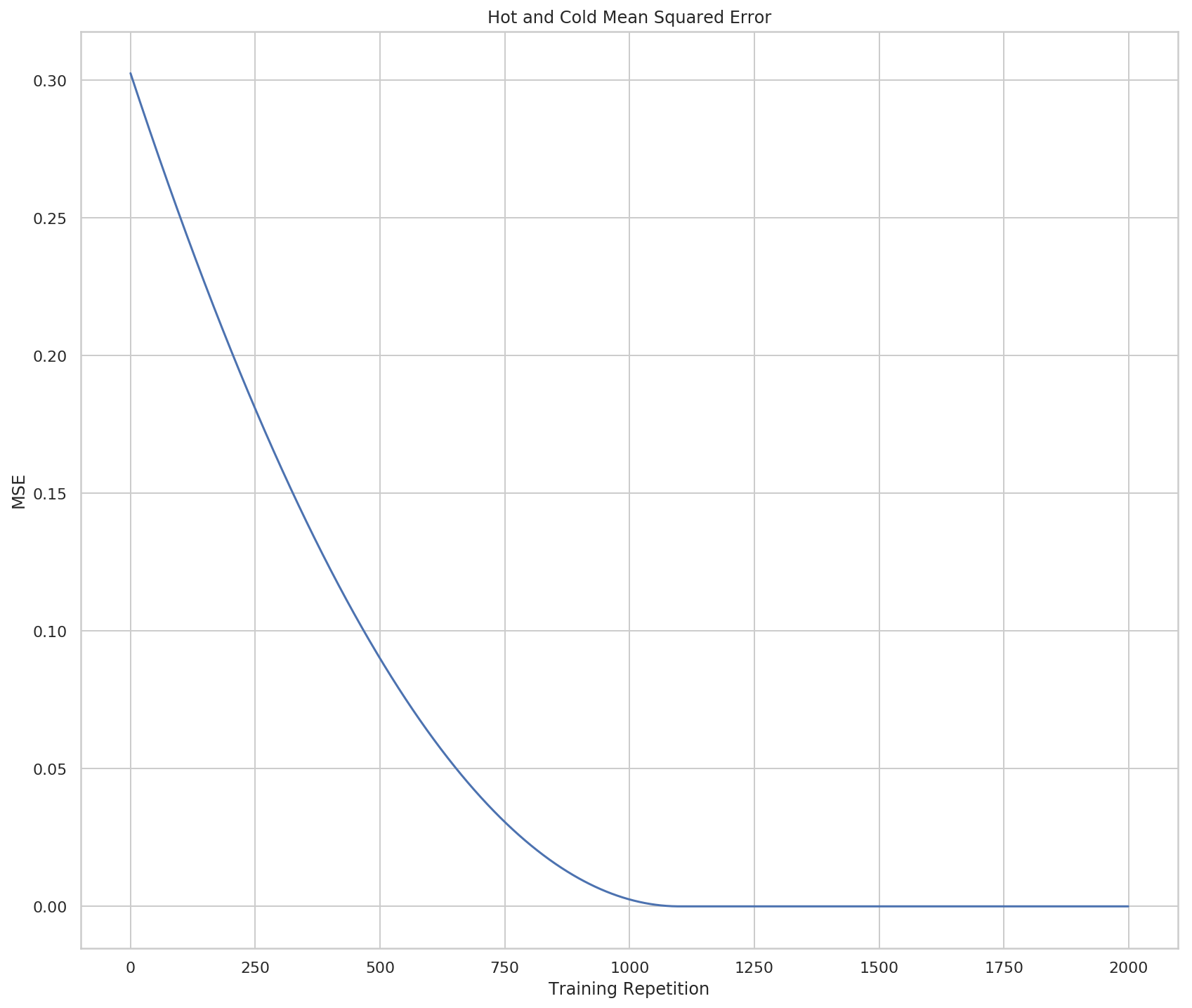
Looking at the output you can see that it reached an error of (nearly) zero at the 1,100th repetition. Based on the plot it looks like it kind of slowed down at the end, which is odd since we're using addition and subtraction, but I guess as the weight gets bigger the proportion of change you add becomes less.
figure, axe = pyplot.subplots(figsize=FIGURE_SIZE)
axe.set_title("Hot and Cold Mean Squared Error vs Weights")
axe.set_xlabel("Weight")
axe.set_ylabel("MSE")
lines = axe.plot(weights, errors, ".")
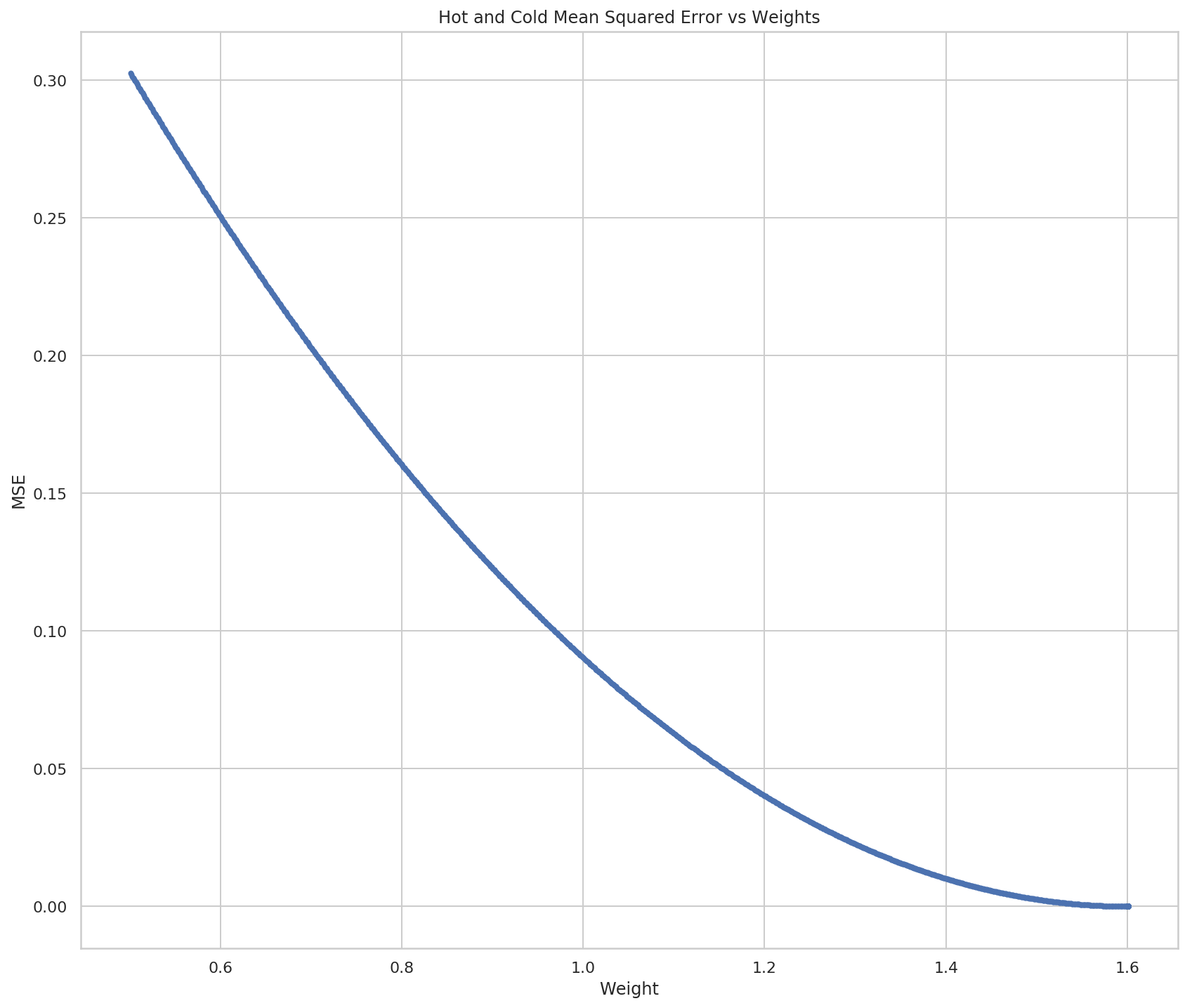
Our optimal weight appears to be 1.6. Given the simplicity of our model we can check by solving the equation.
\[ prediction = weight \times input\\ weight = \frac{prediction}{input} \]
print(prediction/input_value)
1.6009999999999343
So, that looks about right.
Pros and Cons of Hot and Cold Learning
The main thing that Hot and Cold Learning has going for it is that it is simple to understand and implement. There are a couple of problems with it though:
- You have to make multiple predictions per knob to make a decision on the change to make.
- The amount you change the weight at each step can make it impossible to get the right weight, and in most cases you won't have just one input value so it's hard to know what to pick
Is there a better way to update the weights?
With Hot and Cold Learning we make multiple predictions to decide which direction to add a set amount to the weight. But we can instead use the error to change our weight, and in doing so we will change both direction and scale based on the error. In this case error means "pure error", or just the difference between the prediction and the actual value.
\[ error = prediction - actual \]
Since we don't square it the error will be positive if our prediction is too high and negative if it is too low. We don't want to just use the difference, though, because we are adjusting a weight that gets multiplied by the input, so we need to scale the amount of change by the input.
Note that the ordering is now important - you have to subtract the error in the version above and add it if the terms are switched.
\[ adjustment = error * input\\ weights' = weights - adjustment \]
This is the method of Gradient Descent. This is how it looks run on our previous problem.
weight = 0.5
input_value = 0.5
actual = 0.8

prediction = toes_model(input_value, weight)
print_error(prediction, actual, "Step    1 Weight: {}".format(weight), "\t")
errors = []
weights = []
optimal_step = False
tolerance = 0.1**8
optimal_count = 0
print_every = 5
stop_after = 30
for step in range(1, 2001):
    prediction = toes_model(input_value, weight)
    difference = (prediction - actual) * input_value
    weight -= difference
    weights.append(weight)
    error = (print_error(prediction, actual,
                         "Step {:4} Weight: {:.2f}".format(step, weight), "\t")
             if not step % print_every else (prediction - actual)**2)
    errors.append(error)
    if not optimal_step and error < tolerance:
        optimal_step = step - 1
    if error < tolerance:
        optimal_count += 1
    if optimal_count >= stop_after:
        break
print("Optimum Reached at Step {}".format(optimal_step))
Step    1 Weight: 0.5   Predicted: 0.25 Actual: 0.8     MSE: 0.3025
Step    5 Weight: 1.34  Predicted: 0.63 Actual: 0.8     MSE: 0.0303
Step   10 Weight: 1.54  Predicted: 0.76 Actual: 0.8     MSE: 0.0017
Step   15 Weight: 1.59  Predicted: 0.79 Actual: 0.8     MSE: 0.0001
Step   20 Weight: 1.60  Predicted: 0.80 Actual: 0.8     MSE: 0.0000
Step   25 Weight: 1.60  Predicted: 0.80 Actual: 0.8     MSE: 0.0000
Step   30 Weight: 1.60  Predicted: 0.80 Actual: 0.8     MSE: 0.0000
Step   35 Weight: 1.60  Predicted: 0.80 Actual: 0.8     MSE: 0.0000
Step   40 Weight: 1.60  Predicted: 0.80 Actual: 0.8     MSE: 0.0000
Step   45 Weight: 1.60  Predicted: 0.80 Actual: 0.8     MSE: 0.0000
Step   50 Weight: 1.60  Predicted: 0.80 Actual: 0.8     MSE: 0.0000
Step   55 Weight: 1.60  Predicted: 0.80 Actual: 0.8     MSE: 0.0000
Step   60 Weight: 1.60  Predicted: 0.80 Actual: 0.8     MSE: 0.0000
Optimum Reached at Step 30
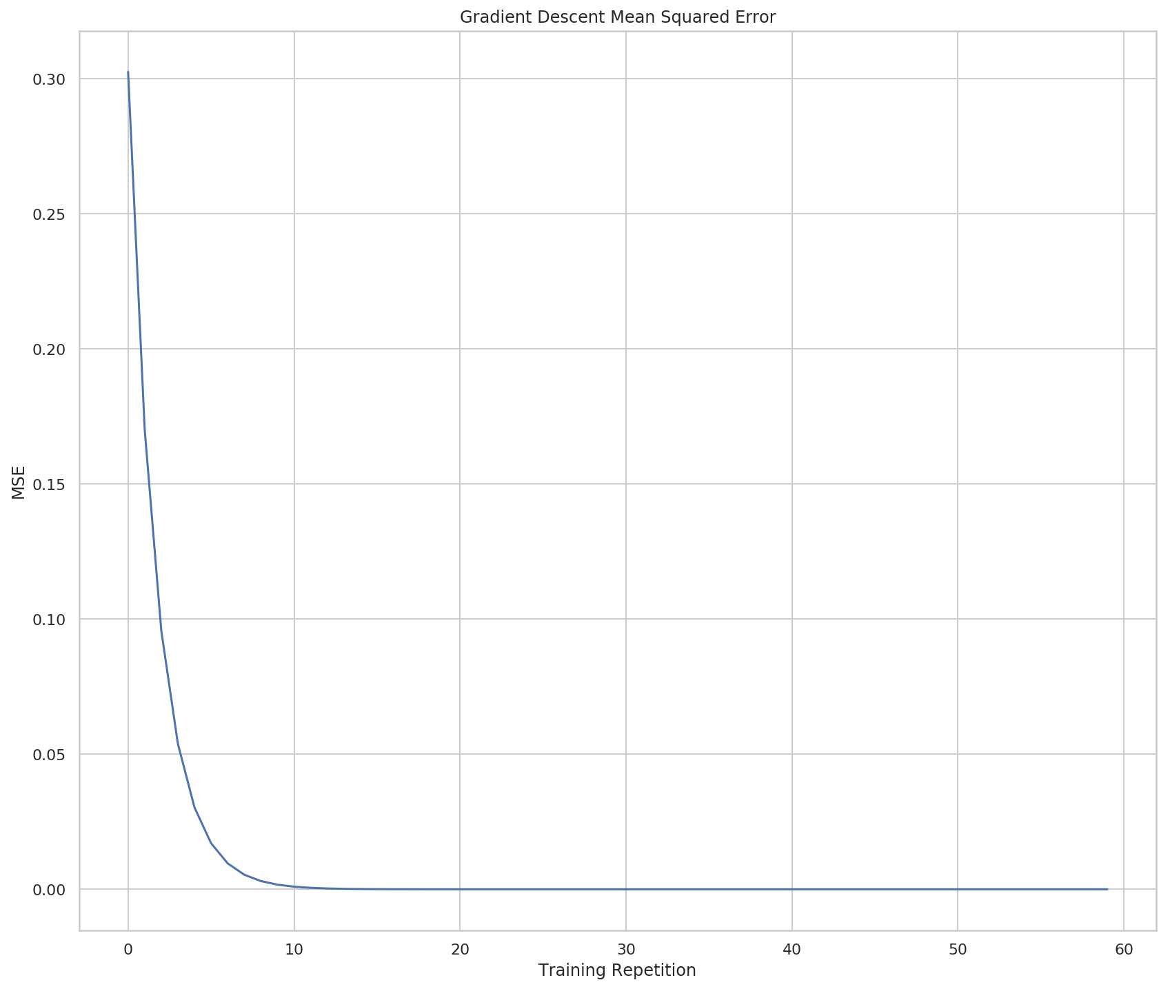
So it now hits the optimal solution at the 30th step instead of the 1,100th step (although it really seems to reach it at step 20, I think the difference is a rounding problem).
figure, axe = pyplot.subplots(figsize=FIGURE_SIZE)
axe.set_title("Gradient Descent Mean Squared Error")
axe.set_xlabel("Training Repetition")
axe.set_ylabel("MSE")
lines = axe.plot(range(len(errors)), errors)
figure, axe = pyplot.subplots(figsize=FIGURE_SIZE)
axe.set_title("Gradient Descent Mean Squared Error vs Weights")
axe.set_xlabel("Weight")
axe.set_ylabel("MSE")
lines = axe.plot(weights, errors, "o")
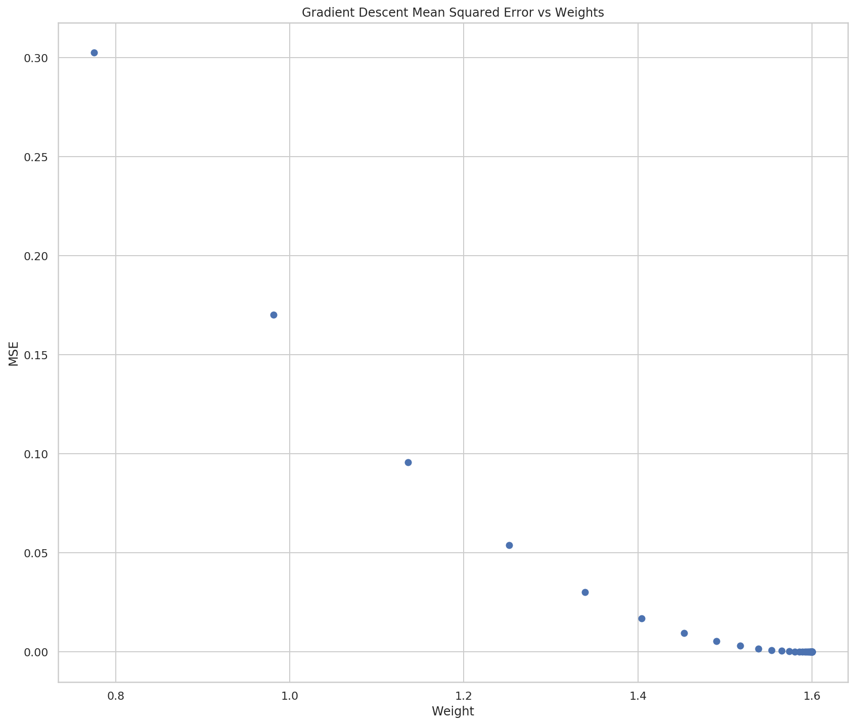
The plots show what we already saw in the output, that Gradient Descent converges on a solution much faster than Hot and Cold Learning does.
Why multiply the error by the input?
This has three main effects called stopping, negative reversal, and scaling.
What is Stopping?
Stopping refers to the case where the input is 0. If that's the case then we don't want to adjust the weight so multiplying the error by the input nullifies it.
What is Negative Reversal?
The sign of the input changes which direction we want the weight to change, so multiplying it by the input keeps the change moving in the right direction even when the sign of the input changes.
What is Scaling?
The larger the input, the greater the amount of change it will add. This can be a bad thing, since the inputs can now have an outsized (negative) effect.
A Discursion On Derivatives
What we're doing when we train our model to minimize our error. In the Mean Squared Error equation:
\[ MSE = \frac{1}{n} \sum_{i=1}^n ((input \times weight) - actual)^2 \]
The only thing we can change is the weight, the input and actual output is set by the data. So what we're interested in is how the error changes as we change the weight. The relationship between how the output changes in relationship to how the input changes is the derivative. One way to think of the derivative is the slope at a point on a line. If you have a straight line the slope will be the same everywhere on it, but if it is curved then different points will have different slopes.
In our case our input is the weight and the output is the error. If you think about slope as \[\frac{rise}{run}\] you'll notice that the bigger the rise, the bigger the slope (since we're taking it at a point the run is infinitesimal), and it's positive going up and negative going down, so if you think of the plot of the MSE earlier, the further you go away from the center (where the error is zero), the steeper the slope, and moving away from the center is always moving up, so the slope is always positive, and moving toward the center where the error is zero is always moving down, so the slope is negative.
What we want, then, is to move our weights in the opposite direction of the slope. There's more math involved to explain this than I can handle right now, but when we calculate our weight adjustment, we are calculating the derivative, and since we want to move in the opposite direction of the derivative, we negate it. And the further away we are from the true value (where our error is zero), the greater the difference is, as we would expect from the slope of our line.
\[ \Delta = prediction - actual\\ \Delta_{weighted} = \Delta \times input\\ weight' = weight - \Delta_{weighted} \]
When does this work?
Well, it's easier to look at when it doesn't work than when it does.
class OneNode:
    """Implements a single-node network

    Args:
     weight: the starting weight for the edge from the input to the output
     input_value: the input to the node
     actual: the actual output we are trying to predict

     training_steps: how many times to train the model
     tolerance: how close to zero we need our error to be
     print_every: how often to print training status
     stop_after: how many times to keep going after the optimal was found
    """
    def __init__(self, weight: float,
                 input_value: float,
                 actual: float,
                 training_steps: int=200,
                 tolerance: float=0.1**8,
                 print_every: int=5, stop_after: int=30) -> None:
        self.original_weight = weight
        self.weight = weight
        self.input_value = input_value
        self.actual = actual
        self.training_steps = training_steps
        self.tolerance = tolerance
        self.print_every = print_every
        self.stop_after = stop_after
        self._errors = None
        self._weights = None
        self._predictions = None
        return

    @property
    def errors(self) -> list:
        """list of MSE values"""
        if self._errors is None:
            self._errors = []
        return self._errors

    @property
    def weights(self) -> list:
        """List of weights built during training"""
        if self._weights is None:
            self._weights = [self.weight]
        return self._weights

    @property
    def predictions(self) -> list:
        """List of predictions made"""
        if self._predictions is None:
            self._predictions = []
        return self._predictions

    @property
    def prediction(self) -> float:
        """The current model's prediction"""
        return self.weight * self.input_value

    def mean_squared_error(self) -> float:
        """The mean squared error for the prediction"""
        try:
            self.predictions.append(self.prediction)
            return (self.prediction - self.actual)**2
        except OverflowError as error:
            print(error)
            print("prediction: {}".format(self.prediction))
            print("actual: {}".format(self.actual))
        return

    def print_error(self,
                    step: int,
                    separator: str="\t",
                    force_print: bool=False,
                    store_error: bool=True) -> float:
        """Prints the (mean) squared error

       Args:
        step: what step this is
        separator: How to separate the output
        force_print: ignore the step count and print anyway
        store_error: whether to add to the errors
       Returns:
        mse: the error
       """
        error = self.mean_squared_error()
        if store_error:
            self.errors.append(error)
        if force_print or not step % self.print_every:
            print("Input: {} Actual Output: {}".format(self.input_value,
                                                       self.actual))
            print(separator.join(["Step: {}".format(step),
                                  "Weight: {}".format(self.weight),
                                  "Predicted: {:.2f}".format(self.prediction),
                                  "MSE: {:.4f}".format(error)]))
        return error

    def adjust_weight(self) -> None:
        """Takes the gradient descent step"""
        scaled_derivative = (self.prediction - self.actual) * self.input_value
        self.weight -= scaled_derivative
        self.weights.append(self.weight)
        return

    def train(self):
        """Trains our model on the values

       """
        self.reset()
        prediction = self.weight * self.input_value
        optimal_step = optimal_count = 0
        error = self.print_error(1,
                                 force_print=True,
                                 store_error=False)
        for step in range(1, self.training_steps + 1):
            error = self.print_error(step)
            if error is None:
                return

            self.adjust_weight()
            if not optimal_step and error < self.tolerance:
                optimal_step = step - 1
            if error < tolerance:
                optimal_count += 1
            if optimal_count >= self.stop_after:
                break
        print("Optimum Reached at Step {}".format(optimal_step))
        return

    def plot_errors_over_time(self, scale="linear") -> None:
        """Plots the error as it is trained

       Args:
        scale: y-axis scale
       """
        figure, axe = pyplot.subplots(figsize=FIGURE_SIZE)
        axe.set_title("Gradient Descent Mean Squared Error")
        axe.set_xlabel("Training Repetition")
        axe.set_ylabel("MSE")
        axe.set_yscale(scale)
        lines = axe.plot(range(len(self.errors)), self.errors)
        return

    def plot_errors_vs_weights(self, style="o") -> None:
        """Plots errors given weights"""
        figure, axe = pyplot.subplots(figsize=FIGURE_SIZE)
        axe.set_title("Gradient Descent Mean Squared Error vs Weights")
        axe.set_xlabel("Weight")
        axe.set_ylabel("MSE")
        lines = axe.plot(self.weights, self.errors, style)
        return

    def plot_weight_distribution(self) -> None:
        """Plots the distribution of the weights"""
        figure, axe = pyplot.subplots(figsize=FIGURE_SIZE)
        axe.set_title("Distribution Of Weights")
        lines = seaborn.distplot(self.weights)
        return


    def reset(self):
        """Resets the properties"""
        self._errors = None
        self._weights = None
        self._predictions = None
        self.weight = self.original_weight
        return
Really Big Inputs
network = OneNode(weight=0.1, input_value=5, actual=0.1, print_every=30)
network.train()
Input: 5 Actual Output: 0.1
Step: 1 Weight: 0.1     Predicted: 0.50 MSE: 0.1600
Input: 5 Actual Output: 0.1
Step: 30        Weight: -8.496029205125367e+38  Predicted: -4248014602562683567255766167412625375232.00 MSE: 18045628063585794511112671022597693816764790617265863683813015097617735965736960.0000
Input: 5 Actual Output: 0.1
Step: 60        Weight: -2.1654753676302967e+80 Predicted: -1082737683815148355196656106977575165473067380893761893846901009426287310965571584.00       MSE: 1172320891953392254658250331342439625964504567088377053437708818301948653571886896236931555371967400274585017142698424782066192956435576184566862647806273773371392.0000
Input: 5 Actual Output: 0.1
Step: 90        Weight: -5.51938258990998e+121  Predicted: -275969129495499010312802960568845701886516344963538842611688052470072992651229004282112996195046030793242534509005731004416.00      MSE: 76158960434503501277477316231095001035615545032300898123025508833954593912013767638712660721529293958181614329406854402338675069139074333788043867020532267345247209268079568592806683870329999393916410491701860464641755145654976460424275531137024.0000
(34, 'Numerical result out of range')
prediction: 1.5336245888098994e+154
actual: 0.1
So, when the input is too big, the prediction explodes.
network.plot_errors_over_time()
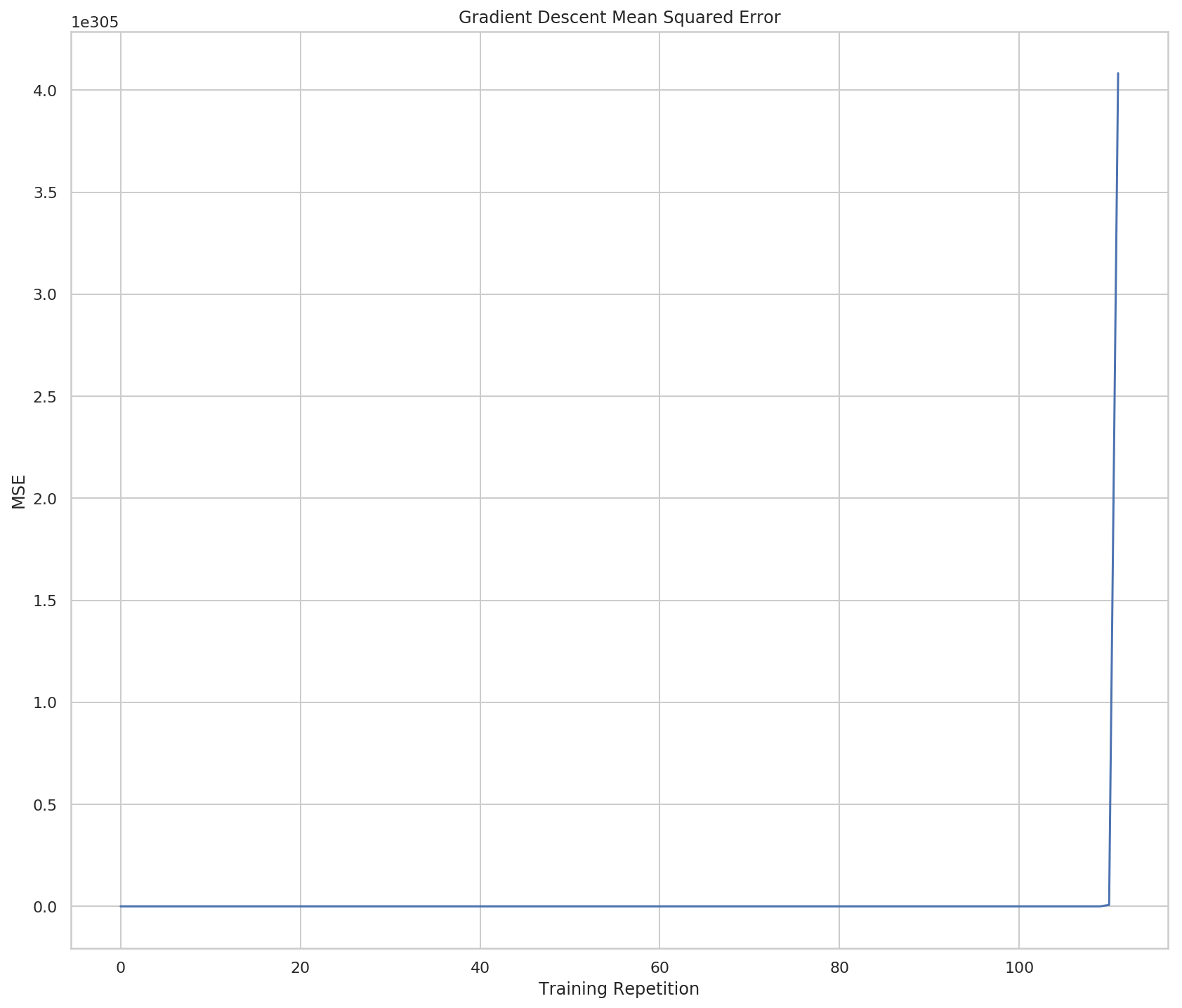
It looks at first like there was no error and then all of a sudden it got huge - but if you look at the scale of the y-axis it maxes out at over \(4\times10^{305}\) and then the overflow error causes it to quit. So when the input is too large, the network goes out of control.
network.plot_errors_vs_weights()
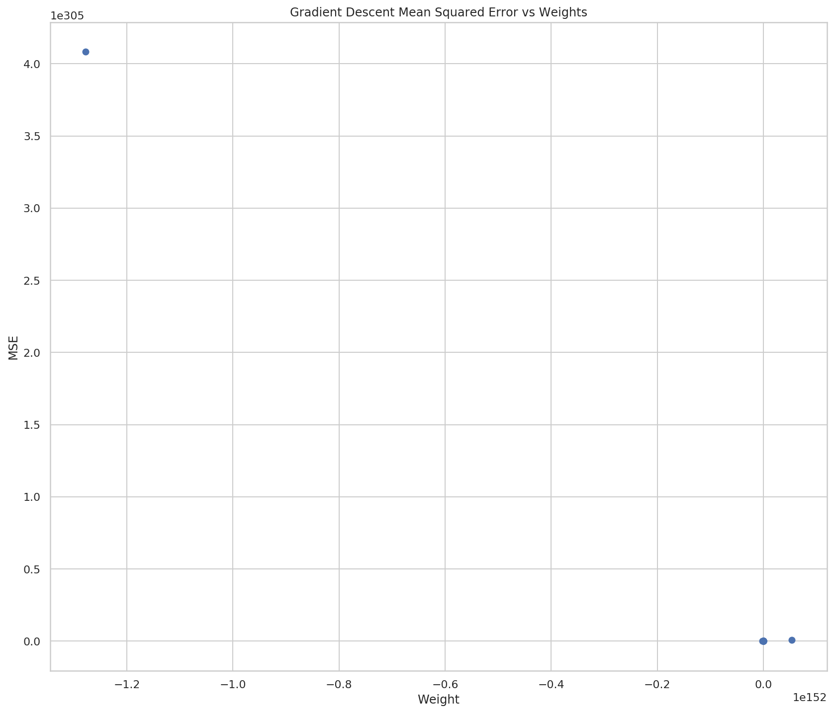 So now it looks like there aren't really many weights, but if you look at both the X and Y scales you can see that they're really huge, so most of the points are probably centered around 0 (relative to the overall scale) and then all of a sudden they go crazy on the last two points.
figure, axe
network.plot_weight_distribution()
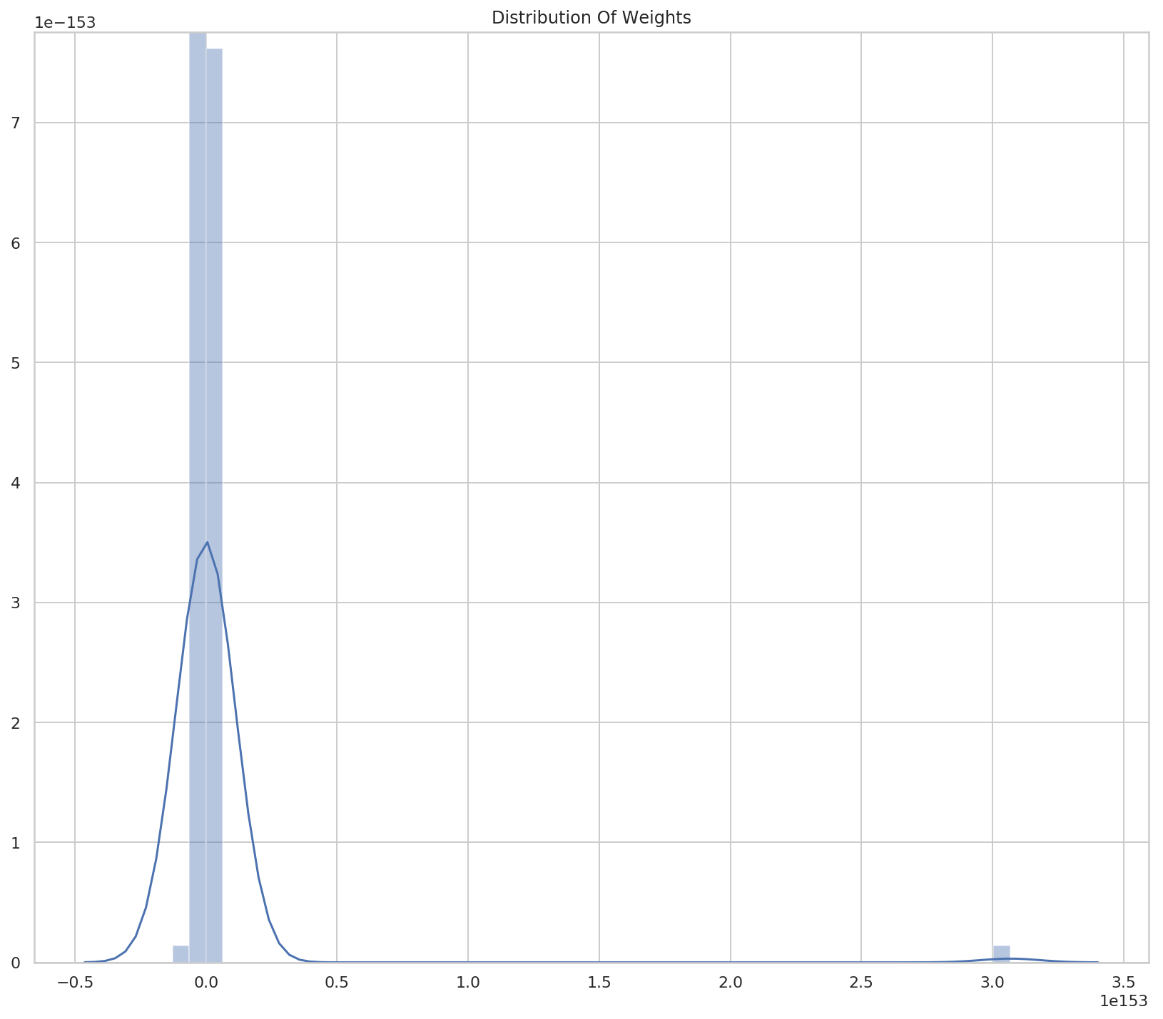
So we have a small number of weights that are very large. Or a lot of very large weights with a small number of very-very-large weights.
weights = pandas.Series(network.weights)
print(weights.describe())
count     1.130000e+02
mean     2.605805e+151
std      2.888965e+152
min     -1.278020e+152
25%      -6.526920e+74
50%      -1.900000e+00
75%       1.566461e+76
max      3.067249e+153
dtype: float64
So the median is -1.9 and the mean is \(0.6 \times 10^{151}\). Looks like there are some outliers.
Fixing the Big Input Problem
The problem with big inputs is that they cause the gradient descent to explode. Remember our error function:
\[ error = input \times (predicted - actual)\\ = input \times ((input \times weights) - actual) \]
If the input is big the error will be big, and since our correction to the weights is based on the error:
\[ weights' = weights - error \]
our weights can start to swing wildly back and forth with the error growing larger and larger and swinginig between positive and negative numbers. The larger the input, the larger the error, the larger the derivative will be in the opposite direction.
The fix is to only update using a fraction of the correction. We find some value (\(\alpha\)) and multiply it by the change to reduce the influence any one change has. How do we find \(\alpha\)? Well, that turns out to be done by trial and error. If your error goes up as you train, then you probably have to make it smaller.
class AlphaNode(OneNode):
    """Incorporates weight update reduction

    Args:
     alpha: amount to weight the update

     weight: the starting weight for the edge from the input to the output
     input_value: the input to the node
     actual: the actual output we are trying to predict

     training_steps: how many times to train the model
     tolerance: how close to zero we need our error to be
     print_every: how often to print training status
     stop_after: how many times to keep going after the optimal was found
    """
    def __init__(self, alpha: float, *args, **kwargs) -> None:
        self.alpha = alpha
        __class__
        super().__init__(*args, **kwargs)
        return

    def adjust_weight(self) -> None:
        """Takes the gradient descent step with alpha weight"""
        scaled_derivative = (self.prediction - self.actual) * self.input_value
        self.weight -= self.alpha * scaled_derivative
        self.weights.append(self.weight)
        return
Why does this help? Our problem is that the large inputs cause the gradient descent to overshoot past the value that would give zero error and by reducing the amount any one change can have we reduce the likelihood that this will happen.
alpha_network = AlphaNode(alpha=0.1, weight=0.5, input_value=5,
                          actual=0.8, print_every=30)
alpha_network.train()
Input: 5 Actual Output: 0.8
Step: 1 Weight: 0.5     Predicted: 2.50 MSE: 2.8900
Input: 5 Actual Output: 0.8
Step: 30        Weight: -43463.41342612052      Predicted: -217317.07   MSE: 47227055374.1942
Input: 5 Actual Output: 0.8
Step: 60        Weight: -8334186242.344855      Predicted: -41670931211.72      MSE: 1736466508118929965056.0000
Input: 5 Actual Output: 0.8
Step: 90        Weight: -1598089039844441.2     Predicted: -7990445199222206.00 MSE: 63847214481773219178788224499712.0000
Input: 5 Actual Output: 0.8
Step: 120       Weight: -3.064352661386353e+20  Predicted: -1532176330693176459264.00   MSE: 2347564308336405932287023519199639310958592.0000
Input: 5 Actual Output: 0.8
Step: 150       Weight: -5.875928686839428e+25  Predicted: -293796434341971398081118208.00      MSE: 86316344832056315635271476663737243674922770633850880.0000
Input: 5 Actual Output: 0.8
Step: 180       Weight: -1.1267155496783526e+31 Predicted: -56335777483917627928853446918144.00 MSE: 3173719824717480263078840848567916525595895306706307529098395648.0000
Optimum Reached at Step 0
Okay, so that still didn't work, maybe if \(\alpha\) was smaller?
alpha_network.alpha = 0.01
alpha_network.train()
Input: 5 Actual Output: 0.8
Step: 1 Weight: 0.5     Predicted: 2.50 MSE: 2.8900
Input: 5 Actual Output: 0.8
Step: 30        Weight: 0.1600809572142104      Predicted: 0.80 MSE: 0.0000
Input: 5 Actual Output: 0.8
Step: 60        Weight: 0.16000001445750855     Predicted: 0.80 MSE: 0.0000
Optimum Reached at Step 34
So now our model is able to reach the correct value again. Can you figure out what the best \(\alpha\) is ahead of time? The magic eight ball says no. At this point in time the best way to find the hyperparameters for machine learning is to try them until you find the ones that perform the best.