MNIST MLP
Table of Contents
Introduction
This is from Udacity's Deep Learning Repository which supports their Deep Learning Nanodegree.
We are going to train a Multi-Layer Perceptron to classify images from the MNIST database of hand-written digits.
We're going to do it using the following steps.
- Load and visualize the data
- Define a neural network
- Train the model
- Evaluate the performance of our trained model on a test dataset
Imports
From Python
from datetime import datetime
From PyPi
from dotenv import load_dotenv
from torchvision import datasets
import matplotlib.pyplot as pyplot
import seaborn
import torch.nn as nn
import torch.nn.functional as F
import torchvision.transforms as transforms
import torch
import numpy
This Project
from neurotic.tangles.data_paths import DataPathTwo
Setup the Plotting
get_ipython().run_line_magic('matplotlib', 'inline')
seaborn.set(style="whitegrid",
            rc={"axes.grid": False,
                "font.family": ["sans-serif"],
                "font.sans-serif": ["Latin Modern Sans", "Lato"],
                "figure.figsize": (8, 6)},
            font_scale=3)
The Data
The Path To the Data
load_dotenv()
path = DataPathTwo(folder_key="MNIST")
print(path.folder)
print(path.folder.exists())
/home/hades/datasets/MNIST
True
Some Settings
Since I downloaded the data earlier for some other exercise forking sub-processes is probably unnecessary, and for the training and testing we'll use a relatively small batch-size of 20.
WORKERS = 0
BATCH_SIZE = 20
A Transform
We're just going to convert the images to tensors.
transform = transforms.ToTensor()
Split Up the Training and Testing Data
train_data = datasets.MNIST(root=path.folder, train=True,
                            download=True, transform=transform)
test_data = datasets.MNIST(root=path.folder, train=False,
                           download=True, transform=transform)
Create the Batch Loaders
train_batches = torch.utils.data.DataLoader(train_data, batch_size=BATCH_SIZE,
                                            num_workers=WORKERS)
test_batches = torch.utils.data.DataLoader(test_data, batch_size=BATCH_SIZE,
                                           num_workers=WORKERS)
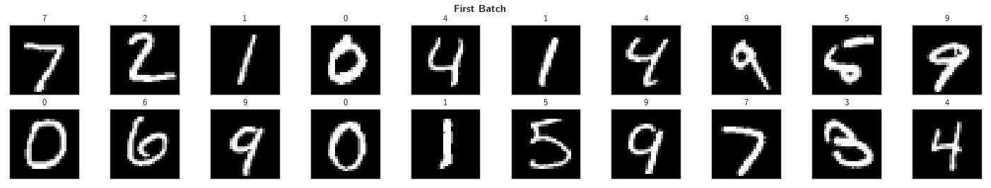
Visualize a Batch of Training Data
The first step in a classification task is to take a look at the data, make sure it is loaded in correctly, then make any initial observations about patterns in that data.
Grab a batch
images, labels = iter(train_batches).next()
images = images.numpy()
Now that we have a batch we're going to plot the images in the batch, along with the corresponding labels.
figure = pyplot.figure(figsize=(25, 4))
figure.suptitle("First Batch", weight="bold")
for index in numpy.arange(BATCH_SIZE):
    ax = figure.add_subplot(2, BATCH_SIZE/2, index+1, xticks=[], yticks=[])
    ax.imshow(numpy.squeeze(images[index]), cmap='gray')
    # print out the correct label for each image
    # .item() gets the value contained in a Tensor
    ax.set_title(str(labels[index].item()))
View a Single Image
Now we're going to take a closer look at the second image in the batch.
image = numpy.squeeze(images[1])

figure = pyplot.figure(figsize = (12,12))
ax = figure.add_subplot(111)
ax.imshow(image, cmap='gray')
width, height = image.shape
threshold = image.max()/2.5
for x in range(width):
    for y in range(height):
        val = round(image[x][y],2) if image[x][y] !=0 else 0
        ax.annotate(str(val), xy=(y,x),
                    horizontalalignment='center',
                    verticalalignment='center',
                    color='white' if image[x][y]<threshold else 'black')
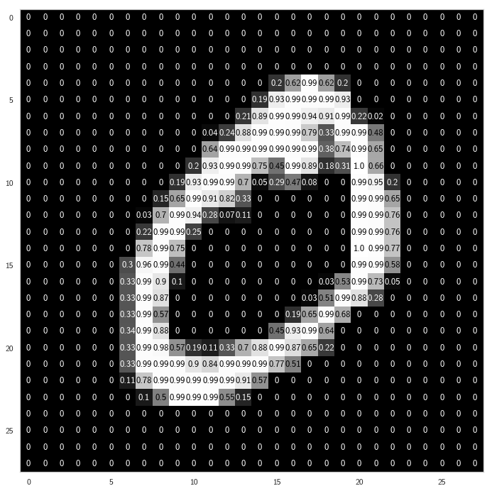
We're looking at a single image with the normalized values for each pixel superimposed on it. It looks like black is 0 and white is 1, although for this image most of the 'white' pixels are just a little less than one.
Define the Network Architecture
The architecture will be responsible for seeing as input a 784-dim Tensor of pixel values for each image, and producing a Tensor of length 10 (our number of classes) that indicates the class scores for an input image. This particular example uses two hidden layers and dropout to avoid overfitting.
These values are based on the keras example implementation.
INPUT_NODES = 28 * 28
HIDDEN_NODES = 512
DROPOUT = 0.2
CLASSES = 10
class Net(nn.Module):
    def __init__(self):
        super().__init__()
        self.fully_connected_layer_1 = nn.Linear(INPUT_NODES, HIDDEN_NODES)
        self.fully_connected_layer_2 = nn.Linear(HIDDEN_NODES, HIDDEN_NODES)
        self.output = nn.Linear(HIDDEN_NODES, CLASSES)
        self.dropout = nn.Dropout(p=DROPOUT)
        return

    def forward(self, x):
        # flatten image input
        x = x.view(-1, 28 * 28)
        # add hidden layer, with relu activation function
        x = self.dropout(F.relu(self.fully_connected_layer_1(x)))
        x = self.dropout(F.relu(self.fully_connected_layer_2(x)))
        return self.output(x)
Initialize the NN
model = Net()
print(model)
Net(
  (fully_connected_layer_1): Linear(in_features=784, out_features=512, bias=True)
  (fully_connected_layer_2): Linear(in_features=512, out_features=512, bias=True)
  (output): Linear(in_features=512, out_features=10, bias=True)
  (dropout): Dropout(p=0.2)
)
A Little CUDA
device = torch.device("cuda" if torch.cuda.is_available() else "cpu")
model.to(device)
Specify the Loss Function and Optimizer
It's recommended that you use cross-entropy loss for classification. If you look at the documentation you can see that PyTorch's cross entropy function applies a softmax function to the output layer and then calculates the log loss (so you don't want to do softmax as part of the model output).
criterion = nn.CrossEntropyLoss()
optimizer = torch.optim.SGD(model.parameters(), lr=0.01)
Train the Network
The steps for training/learning from a batch of data are:
- Clear the gradients of all optimized variables
- Forward pass: compute predicted outputs by passing inputs to the model
- Calculate the loss
- Backward pass: compute gradient of the loss with respect to model parameters
- Perform a single optimization step (parameter update)
- Update average training loss
The following loop trains for 30 epochs; feel free to change this number. For now, we suggest somewhere between 20-50 epochs. As you train, take a look at how the values for the training loss decrease over time. We want it to decrease while also avoiding overfitting the training data.
EPOCHS = 30
start = datetime.now()
model.train() # prep model for training

for epoch in range(EPOCHS):
    # monitor training loss
    train_loss = 0.0
    train_losses = []
    # train the model
    for data, target in train_batches:
        # move it to the GPU or CPU
        data, target = data.to(device), target.to(device)
        # clear the gradients of all optimized variables
        optimizer.zero_grad()
        # forward pass: compute predicted outputs by passing inputs to the model
        output = model(data)
        # calculate the loss
        loss = criterion(output, target)
        # backward pass: compute gradient of the loss with respect to model parameters
        loss.backward()
        # perform a single optimization step (parameter update)
        optimizer.step()
        # update running training loss
        train_loss += loss.item() * data.size(0)

        # print training statistics
        # calculate average loss over an epoch
    train_loss = train_loss/len(train_batches.dataset)
    train_losses.append(train_loss)
    print('Epoch: {} \tTraining Loss: {:.6f}'.format(
        epoch+1,
        train_loss
        ))
print("Training Time: {}".format(datetime.now() - start))
Epoch: 1        Training Loss: 0.826836
Epoch: 2        Training Loss: 0.324859
Epoch: 3        Training Loss: 0.251608
Epoch: 4        Training Loss: 0.202294
Epoch: 5        Training Loss: 0.170231
Epoch: 6        Training Loss: 0.146775
Epoch: 7        Training Loss: 0.127352
Epoch: 8        Training Loss: 0.115026
Epoch: 9        Training Loss: 0.104332
Epoch: 10       Training Loss: 0.093575
Epoch: 11       Training Loss: 0.084913
Epoch: 12       Training Loss: 0.077826
Epoch: 13       Training Loss: 0.071506
Epoch: 14       Training Loss: 0.067273
Epoch: 15       Training Loss: 0.063749
Epoch: 16       Training Loss: 0.058150
Epoch: 17       Training Loss: 0.054770
Epoch: 18       Training Loss: 0.051584
Epoch: 19       Training Loss: 0.047762
Epoch: 20       Training Loss: 0.045219
Epoch: 21       Training Loss: 0.041732
Epoch: 22       Training Loss: 0.040526
Epoch: 23       Training Loss: 0.038247
Epoch: 24       Training Loss: 0.035713
Epoch: 25       Training Loss: 0.033801
Epoch: 26       Training Loss: 0.031963
Epoch: 27       Training Loss: 0.031082
Epoch: 28       Training Loss: 0.028971
Epoch: 29       Training Loss: 0.027500
Epoch: 30       Training Loss: 0.026876
Training Time: 0:05:59.808071
Test the Trained Network
Finally, we test our best model on previously unseen test data and evaluate it's performance. Testing on unseen data is a good way to check that our model generalizes well. It may also be useful to be granular in this analysis and take a look at how this model performs on each class as well as looking at its overall loss and accuracy.
model.eval()
model.eval() will set all the layers in your model to evaluation mode. This affects layers like dropout layers that turn "off" nodes during training with some probability, but should allow every node to be "on" for evaluation!
Set Up the Testing
test_loss = 0.0
class_correct = list(0. for i in range(10))
class_total = list(0. for i in range(10))
model.eval()

start = datetime.now()

for data, target in test_batches:
    data, target = data.to(device), target.to(device)
    # forward pass: compute predicted outputs by passing inputs to the model
    output = model(data)
    # calculate the loss
    loss = criterion(output, target)
    # update test loss
    test_loss += loss.item() * data.size(0)
    # convert output probabilities to predicted class
    _, prediction = torch.max(output, 1)
    # compare predictions to true label
    correct = numpy.squeeze(prediction.eq(target.data.view_as(prediction)))
    # calculate test accuracy for each object class
    for i in range(BATCH_SIZE):
        label = target.data[i]
        class_correct[label] += correct[i].item()
        class_total[label] += 1

print("Test Time: {}".format(datetime.now() - start))
Test Time: 0:00:01.860151
Calculate and Print Average Test Loss
test_loss = test_loss/len(test_batches.dataset)
print('Test Loss: {:.6f}\n'.format(test_loss))

for i in range(10):
    if class_total[i] > 0:
        print('Test Accuracy of Batch {}: {:.2f} ({}/{})'.format(
            str(i), 100 * class_correct[i] / class_total[i],
            numpy.sum(class_correct[i]), numpy.sum(class_total[i])))
    else:
        print('Test Accuracy of {}: N/A (no training examples)'.format(classes[i]))

print('\nTest Accuracy (Overall): %2d%% (%2d/%2d)' % (
    100. * numpy.sum(class_correct) / numpy.sum(class_total),
    numpy.sum(class_correct), numpy.sum(class_total)))
Test Loss: 0.056054

Test Accuracy of Batch 0: 99.18 (972.0/980.0)
Test Accuracy of Batch 1: 99.21 (1126.0/1135.0)
Test Accuracy of Batch 2: 98.16 (1013.0/1032.0)
Test Accuracy of Batch 3: 98.02 (990.0/1010.0)
Test Accuracy of Batch 4: 98.47 (967.0/982.0)
Test Accuracy of Batch 5: 98.43 (878.0/892.0)
Test Accuracy of Batch 6: 98.12 (940.0/958.0)
Test Accuracy of Batch 7: 97.47 (1002.0/1028.0)
Test Accuracy of Batch 8: 97.13 (946.0/974.0)
Test Accuracy of Batch 9: 98.12 (990.0/1009.0)

Test Accuracy (Overall): 98% (9824/10000)
Visualize Sample Test Results
This cell displays test images and their labels in this format: predicted (ground-truth). The text will be green for accurately classified examples and red for incorrect predictions.
Obtain One Batch of Test Images
model.cpu()
dataiter = iter(test_batches)
images, labels = dataiter.next()

# get sample outputs
output = model(images)
# convert output probabilities to predicted class
_, preds = torch.max(output, 1)
# prep images for display
images = images.numpy()
# plot the images in the batch, along with predicted and true labels
fig = pyplot.figure(figsize=(25, 4))
for idx in numpy.arange(20):
    ax = fig.add_subplot(2, 20/2, idx+1, xticks=[], yticks=[])
    ax.imshow(numpy.squeeze(images[idx]), cmap='gray')
    ax.set_title("{} ({})".format(str(preds[idx].item()), str(labels[idx].item())),
                 color=("green" if preds[idx]==labels[idx] else "red"))
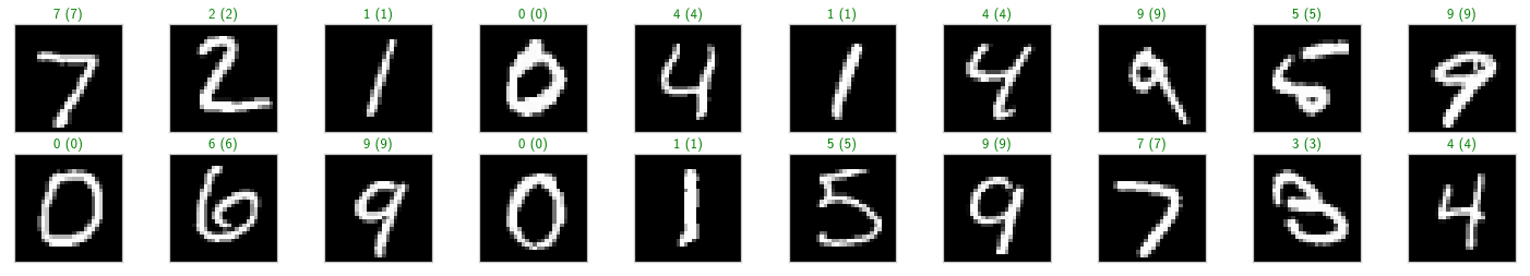
This model is surprisingly accurate. I say surprising, even though we created a very accurate model previously, because in my original implementation I used RMSprop as the optimizer, because that's what the Keras implementation used, but then I only got 11%. I'm guessing that there's some extra tuning you need to do to the parameters for RMSprop but I just naively used the defaults. In any case, it semms that SGD is still the champ.