Part 4 - Classifying Fashion-MNIST

Cloistered Monkey

2018-11-19 19:15

Introduction

This is from Udacity's Deep Learning Repository which supports their Deep Learning Nanodegree.

This post uses the Fashion-MNIST dataset, a set of article images from Zalando, a fashion retailer. It is meant to be a drop-in replacement for the MNIST dataset. The dataset was created because some people the consider original MNIST too easy, with classical machine learning algorithms achieving better than 97% accuracy. The dataset keeps the 10 classes, but now instead of digits they represent clothing types.

Label	Description
0	T-shirt/top
1	Trouser
2	Pullover
3	Dress
4	Coat
5	Sandal
6	Shirt
7	Sneaker
8	Bag
9	Ankle boot

descriptions = ("T-shirt/top",
                "Trouser",
                "Pullover",
                "Dress",
                "Coat",
                "Sandal",
                "Shirt",
                "Sneaker",
                "Bag",
                "Ankle boot",
                )

label_decoder = dict(zip(range(10), descriptions))

Set Up

Imports

Python Standard Library

from collections import OrderedDict

PyPi

from torchvision import datasets, transforms
from torch import nn, optim
import seaborn
import torch
import torch.nn.functional as F

The Udacity Code

from nano.pytorch import helper

Plotting

get_ipython().run_line_magic('matplotlib', 'inline')
get_ipython().run_line_magic('config', "InlineBackend.figure_format = 'retina'")
seaborn.set(style="whitegrid",
            rc={"axes.grid": False,
                "font.family": ["sans-serif"],
                "font.sans-serif": ["Latin Modern Sans", "Lato"],
                "figure.figsize": (8, 6)},
            font_scale=1)

The Data

Normalization

First, a transform to normalize the data.

means = (0.5, 0.5, 0.5)
deviations = means
transform = transforms.Compose([transforms.ToTensor(),
                                transforms.Normalize(means, deviations)])

Load The Data

First our training set.

training = datasets.FashionMNIST('~/datasets/F_MNIST/',
                                 download=True,
                                 train=True,
                                 transform=transform)

training_batches = torch.utils.data.DataLoader(training,
                                               batch_size=64,
                                               shuffle=True)

Downloading http://fashion-mnist.s3-website.eu-central-1.amazonaws.com/train-images-idx3-ubyte.gz
Downloading http://fashion-mnist.s3-website.eu-central-1.amazonaws.com/train-labels-idx1-ubyte.gz
Downloading http://fashion-mnist.s3-website.eu-central-1.amazonaws.com/t10k-images-idx3-ubyte.gz
Downloading http://fashion-mnist.s3-website.eu-central-1.amazonaws.com/t10k-labels-idx1-ubyte.gz
Processing...
Done!

Now our test set.

testing = datasets.FashionMNIST('~/datasets/F_MNIST/',
                                download=True,
                                train=False,
                                transform=transform)

test_batches = torch.utils.data.DataLoader(testing,
                                           batch_size=64,
                                           shuffle=True)

The data is apparently on a european amazon web-service server.

Let's take a look at one of the images.

def show_next_image(data_set: torch.utils.data.DataLoader) -> tuple:
    """plots the next image

    Args:
     data_set: iterator to get the next image from

    Returns:
     image, label: the next items in the data set
    """
    image, label = iter(data_set).next()
    helper.imshow(image[0, :])
    return image, label

with seaborn.axes_style(style="white", rc={"figure.figsize": (4, 2)}):
    image, label = show_next_image(training_batches)

Every time I re-run this the image changes. That was originally just a blob.

print(label_decoder[label[0].item()])

Sneaker

The Network

Here you should define your network. As with MNIST, each image is 28x28 which is a total of 784 pixels, and there are 10 classes. You should include at least one hidden layer. We suggest you use ReLU activations for the layers and to return the logits or log-softmax from the forward pass. It's up to you how many layers you add and the size of those layers.

Hyper Parameters

class HyperParameters:
    inputs = 28 * 28
    hidden_layer_1 = 128
    hidden_layer_2 = 64
    outputs = 10
    learning_rate = 0.005
    rows = 1
    epochs = 200

The Model

model = nn.Sequential(
    OrderedDict(
        input_to_hidden=nn.Linear(HyperParameters.inputs,
                                  HyperParameters.hidden_layer_1),
        activation_1=nn.ReLU(),
        hidden_to_hidden=nn.Linear(HyperParameters.hidden_layer_1,
                                   HyperParameters.hidden_layer_2),
        activation_2=nn.ReLU(),
        hidden_to_output=nn.Linear(HyperParameters.hidden_layer_2,
                                   HyperParameters.outputs),
        activation_out=nn.LogSoftmax(dim=HyperParameters.rows),
    )
)

The Optimizer and Loss

criterion = nn.NLLLoss()
optimizer = optim.SGD(model.parameters(), lr=HyperParameters.learning_rate)

Training

The process:

Make a forward pass through the network to get the logits
Use the logits to calculate the loss
Perform a backward pass through the network with `loss.backward()` to calculate the gradients
Take a step with the optimizer to update the weights

By adjusting the hyperparameters (hidden units, learning rate, etc), you should be able to get the training loss below 0.4.

for epoch in range(HyperParameters.epochs):
    running_loss = 0
    for images, labels in training_batches:
        # some setup
        ## Flatten the images
        images = images.view(images.shape[0], -1)
        ## Reset the optimizer
        optimizer.zero_grad()

        # forward pass
        output = model.forward(images)

        # back-propagation
        loss = criterion(output, labels)
        loss.backward()

        # take the next step
        optimizer.step()
        running_loss += loss.item()
    if not epoch % 10:
        print(f"Training loss: {running_loss/len(data_batches)}")

Training loss: 1.2992842076048414
Training loss: 0.4147487568385057
Training loss: 0.3563503011393903
Training loss: 0.31974349495793963
Training loss: 0.2909906929267495
Training loss: 0.2669587785135836
Training loss: 0.24693025264150298
Training loss: 0.22828677767661334
Training loss: 0.2111341437932525
Training loss: 0.19651830268662368
Training loss: 0.18078892016763498
Training loss: 0.1678272306934984
Training loss: 0.15590339134147427
Training loss: 0.1440456182614509
Training loss: 0.13368237831159188
Training loss: 0.1232291767592115
Training loss: 0.11354898248336462
Training loss: 0.104927517529299
Training loss: 0.09589472461912806
Training loss: 0.08939716171846589

Check out a prediction.

images, labels = iter(test_batches).next()
image, label = images[0], labels[0]
# Convert 2D image to 1D vector
image = image.resize_(1, 784)

with torch.no_grad():
    logits = model(image)

probabilities = F.softmax(logits, dim=1)

with seaborn.axes_style(style="whitegrid"):
    helper.view_classify(image.resize_(1, 28, 28), probabilities,
                         version='Fashion')

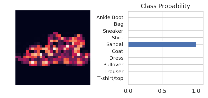
That looks pretty good to me.

print(label_decoder[label.item()])
print(label_decoder[probabilities.argmax().item()])

Sandal
Sandal

So this time we got it right.

for index, label in enumerate(labels):
    if label.item() == 4:
        break
print(index)
image = images[index].resize_(1, 784)
output = model(image)
probabilities = F.softmax(output, dim=1)
print(label_decoder[probabilities.argmax().item()])
print(label_decoder[label.item()])

10
Dress
Coat

Oops, look like we're still having problems.

correct = 0
total = 0
with torch.no_grad():
    for images, labels in test_batches:
        images = images.view(images.shape[0], -1)
        outputs = model(images)
        _, predicted = torch.max(outputs.data, 1)
        total += labels.size(0)
        correct += (predicted == labels).sum().item()

print('Accuracy of the network on the test images: %d %%' % (
    100 * correct / total))

Accuracy of the network on the test images: 88 %

Not bad, it could probably be tuned to do better, the loss hasn't stopped reducing, for instance, so maybe more epochs would help.

class_correct = list(0. for i in range(10))
class_total = list(0. for i in range(10))
print("|Item|Accuracy (%)|")
print("|-+-|")
with torch.no_grad():
    for images, labels in test_batches:
        images = images.view(images.shape[0], -1)
        outputs = model(images)
        _, predicted = torch.max(outputs, 1)
        c = (predicted == labels).squeeze()
        for i in range(len(labels)):
            label = labels[i]
            class_correct[label.item()] += c[i].item()
            class_total[label.item()] += 1


for i in range(10):
    print('|{}|{:.1f}'.format(
        label_decoder[i], 100 * class_correct[i] / class_total[i]))

Item	Accuracy (%)
T-shirt/top	88.0
Trouser	97.5
Pullover	87.2
Dress	88.0
Coat	83.2
Sandal	97.4
Shirt	57.3
Sneaker	95.5
Bag	95.7
Ankle boot	95.6

Generally it seems to do okay, but the shirt seems to have gotten worse than when I was using fewer epochs. I might be overfitting by putting so many epochs and if I were to improve it I would probably work on other hyper-parameters.

Table of Contents