In this assignment you will train several models and evaluate how effectively they predict instances of credit-card fraud using data based on this dataset from Kaggle. This is their description:
The datasets contains transactions made by credit cards in September 2013 by european cardholders. This dataset presents transactions that occurred in two days, where we have 492 frauds out of 284,807 transactions. The dataset is highly unbalanced, the positive class (frauds) account for 0.172% of all transactions.

It contains only numerical input variables which are the result of a PCA transformation. Unfortunately, due to confidentiality issues, we cannot provide the original features and more background information about the data. Features V1, V2, ... V28 are the principal components obtained with PCA, the only features which have not been transformed with PCA are 'Time' and 'Amount'. Feature 'Time' contains the seconds elapsed between each transaction and the first transaction in the dataset. The feature 'Amount' is the transaction Amount, this feature can be used for example-dependant cost-senstive learning. Feature 'Class' is the response variable and it takes value 1 in case of fraud and 0 otherwise.

Given the class imbalance ratio, we recommend measuring the accuracy using the Area Under the Precision-Recall Curve (AUPRC). Confusion matrix accuracy is not meaningful for unbalanced classification.

The dataset has been collected and analysed during a research collaboration of Worldline and the Machine Learning Group (`http://mlg.ulb.ac.be <http://mlg.ulb.ac.be>`_) of ULB (Université Libre de Bruxelles) on big data mining and fraud detection. More details on current and past projects on related topics are available on `http://mlg.ulb.ac.be/BruFence <http://mlg.ulb.ac.be/BruFence>`_ and `http://mlg.ulb.ac.be/ARTML <http://mlg.ulb.ac.be/ARTML>`_

Please cite: Andrea Dal Pozzolo, Olivier Caelen, Reid A. Johnson and Gianluca Bontempi. Calibrating Probability with Undersampling for Unbalanced Classification. In Symposium on Computational Intelligence and Data Mining (CIDM), IEEE, 2015
Each row in `fraud_data.csv` corresponds to a credit card transaction. Features include confidential variables `V1` through `V28` as well as `Amount` which is the amount of the transaction.
The target is stored in the `class` column, where a value of 1 corresponds to an instance of fraud and 0 corresponds to an instance of not fraud.
1 Imports
import numpy
import pandas
import matplotlib.pyplot as plot
import seaborn

from sklearn.model_selection import (
    GridSearchCV,
    train_test_split,
    )
from sklearn.svm import SVC
from sklearn.dummy import DummyClassifier
from sklearn.linear_model import LogisticRegression
from sklearn.metrics import (
    auc,
    confusion_matrix,
    precision_recall_curve,
    precision_score,
    recall_score,
    roc_curve,
    )
from tabulate import tabulate
DATA = "data/fraud_data.csv"
2 Setup the plotting
get_ipython().magic('matplotlib inline')
style = seaborn.axes_style("whitegrid")
style["axes.grid"] = False
seaborn.set_style("whitegrid", style)
3 Exploring the data
3.1 How much fraud is there?
Import the data from `fraud_data.csv`. What percentage of the observations in the dataset are instances of fraud?
data = pandas.read_csv(DATA)
print("Fraction of cases that were fraud: {0:.2f}".format(data.Class.sum()/data.Class.count()))
Fraction of cases that were fraud: 0.02
seaborn.countplot(x="Class", data=data)

So it appears that most of the cases aren't fraudulent.
4 Setting up the training and testing sets
As always, we split the data into training and testing sets so there's no `data leakage`.
data = pandas.read_csv(DATA)

X = data.iloc[:,:-1]
y = data.iloc[:,-1]

X_train, X_test, y_train, y_test = train_test_split(X, y, random_state=0)
5 Scores
This is a convenience class to store the scores for the models.
class ScoreKeeper(object):
    """only holds scores, doesn't create them"""
    def __init__(self):
        self.precision = "N/A"
        self.accuracy = "N/A"
        self.recall = "N/A"
        return

    def __sub__(self, other):
        """calculates the difference between the three scores

        Args:
         other (Scores): the right-hand side of the subtraction

        Returns:
         ScoreKeeper: object with the differences

        Raises:
         TypeError: one of the values wasn't set on one of the Scores
        """
        scores = ScoreKeeper()
        scores.accuracy = self.accuracy - other.accuracy
        scores.precision = self.precision - other.precision
        scores.recall = self.recall - other.recall
        return scores

    def __gt__(self, other):
        """compares scores

        Args:
         other (Scores): object to compare to

        Returns:
         bool: True if all three scores are greater than other's

        Raises:
         TypeError: one of the values wasn't set
        """
        return all((self.accuracy > other.accuracy,
                    self.precision > other.precision,
                    self.recall > other.recall))

    def __str__(self):
        return "Precision: {0:.2f}, Accuracy: {1:.2f}, Recall: {2:.2f}".format(
            self.precision,
            self.accuracy,
            self.recall)
class Scores(ScoreKeeper):
    """holds scores"""
    def __init__(self, model, x_test, y_test):
        """fits and scores the model

        Args:
         model: model that has been fit to the data
         x_test: input for accuracy measurement
         y_test: labels for scoring the model
        """
        self.x_test = x_test
        self.y_test = y_test
        self._accuracy = None
        self._recall = None
        self._precision = None
        self.model = model
        self._predictions = None
        self._scores = None
        return

    @property
    def predictions(self):
        """the model's predictions

        Returns:
         array: predictions for x-test
        """
        if self._predictions is None:
            self._predictions = self.model.predict(self.x_test)
        return self._predictions

    @property
    def accuracy(self):
        """the accuracy of the model's predictions

        the fraction that was correctly predicted

        (tp + tn)/(tp + tn + fp + fn)

        Returns:
         float: accuracy of predictions for x-test
        """
        if self._accuracy is None:
            self._accuracy = self.model.score(self.x_test, self.y_test)
        return self._accuracy

    @property
    def recall(self):
        """the recall score for the predictions

        The fraction of true-positives penalized for missing any
        This is the better metric when missing a case is more costly
        than accidentally identifying a case.

        tp / (tp + fn)

        Returns:
         float: recall of the predictions
        """
        if self._recall is None:
            self._recall = recall_score(self.y_test, self.predictions)
        return self._recall

    @property
    def precision(self):
        """the precision of the test predictions

        The fraction of true-positives penalized for false-positives
        This is the better metric when accidentally identifying a case
        is more costly than missing a case

        tp / (tp + fp)

        Returns:
         float: precision score
        """
        if self._precision is None:
            self._precision = precision_score(self.y_test, self.predictions)
        return self._precision
6 A Dummy Classifier (baseline)
Using `X_train`, `X_test`, `y_train`, and `y_test` (as defined above), we're going to train a dummy classifier that classifies everything as the majority class of the training data, so we will have a baseline to compare with the other models.
First we create and train it
strategy = "most_frequent"
dummy = DummyClassifier(strategy=strategy)
dummy.fit(X_train, y_train)
dummy_scores = Scores(dummy, X_test, y_test)
Now we make our predctions and score them
print("Dummy Classifier: {0}".format(dummy_scores))
Dummy Classifier: Precision: 0.00, Accuracy: 0.99, Recall: 0.00
Since the model is always predicting that the data-points are not fraudulent (the majority case), it never returns any true positives and since both precision and recall have true positive as their numerators, they are both 0.
For the accuracy we can look at the count of each class:
y_test.value_counts()
0    5344
1      80
Name: Class, dtype: int64
And since we know it will always predict 0, we can double-check it (the true and false positives are both 0).
true_positive = 0
true_negative = 5344
false_positive = 0
false_negative = 80
accuracy = (true_positive + true_negative)/(true_positive + true_negative
                                            + false_positive + false_negative)
print("Accuracy: {0:.2f}".format(accuracy))
assert round(accuracy, 2) == round(dummy_scores.accuracy, 2)
Accuracy: 0.99
7 SVC Accuracy, Recall and Precision
Now we're going to create a Support Vector Classifier that uses the sklearn default valuse.
svc = SVC()
svc.fit(X_train, y_train)
svc_scores = Scores(svc, X_test, y_test)
print("SVC: {0}".format(svc_scores))
SVC: Precision: 1.00, Accuracy: 0.99, Recall: 0.38
We can now compare it to the Dummy Classifier to see how it did against the baseline.
print("SVC - Dummy: {0}".format(svc_scores - dummy_scores))
assert svc_scores > dummy_scores
SVC - Dummy: Precision: 1.00, Accuracy: 0.01, Recall: 0.38
The SVC was much better on precision and recall (as expected) and slightly better on accuracy.
8 Confusion Matrix
We're going to create a Support Vector Classifier with ``C=1e9`` and ``gamma=1e-07`` (the ``e`` is the equivalent of ``**``). Then, using the decision function and a threshold of -220, we're going to make our predictions and create a confusion matrix. The decision-function calculates the distance of each data point from the label, so the further a value is from 0, the further it is from the separating hyper-plane.
error_penalty = 1e9
kernel_coefficient = 1e-07
threshold = -220
svc_2 = SVC(C=error_penalty, gamma=kernel_coefficient)
svc_2.fit(X_train, y_train)
svc_scores_2 = Scores(svc_2, X_test, y_test)
The decision_function gives us the distances which we then need to convert to labels. In this case we're going to label anything greater than -220 as a 1 and anything less as a 0.
decisions = svc_2.decision_function(X_test)
decisions[decisions > threshold] = 1
decisions[decisions != 1] = 0
matrix = confusion_matrix(y_test, decisions)
matrix = pandas.DataFrame(matrix, index=["Actual Positive", "Actual Negative"], columns = ["Predicted Positive", "Predicted Negative"])
print(tabulate(matrix, tablefmt="orgtbl",
               headers="keys"))
|
Predicted Positive |
Predicted Negative |
| Actual Positive |
5320 |
24 |
| Actual Negative |
14 |
66 |
print("SVC 2: {0}".format(svc_scores_2))
assert svc_scores_2 > dummy_scores
SVC 2: Precision: 0.94, Accuracy: 1.00, Recall: 0.80
print("SVC 2 - SVC Default: {0}".format(svc_scores_2 - svc_scores))
SVC 2 - SVC Default: Precision: -0.06, Accuracy: 0.01, Recall: 0.43
This model did slightly worse with precision that the default, slightly better for accuracy but quite a bit better for recall. So if we didn't care as much about false positives it would be the better model.
9 Logistic Regression
This model will be a Logistic Regression model built with the default parameters.
For the logisitic regression classifier, we'll create a precision recall curve and a roc curve using y_test and the probability estimates for X_test (probability it is fraud).
Looking at the precision recall curve, what is the recall when the precision is `0.75`?
Looking at the roc curve, what is the true positive rate when the false positive rate is `0.16`?
model = LogisticRegression()
model.fit(X_train, y_train)
y_scores = model.decision_function(X_test)
precision, recall, thresholds = precision_recall_curve(y_test, y_scores)
closest_zero = numpy.argmin(numpy.abs(thresholds))
closest_zero_precision = precision[closest_zero]
closest_zero_recall = recall[closest_zero]
index = numpy.where(precision==0.75)[0][0]
recall_at_precision = recall[index]
figure = plot.figure()
axe = figure.gca()
axe.plot(precision, recall, label="Precision-Recall Curve")
axe.plot(closest_zero_precision, closest_zero_recall, "o", markersize=12, mew=3, fillstyle='none')
axe.set_xlabel("Precision")
axe.set_ylabel("Recall")
axe.axhline(recall_at_precision, color="r")
axe.legend()
title = axe.set_title("Precision vs Recall")

index = numpy.where(precision==0.75)[0][0]
recall_at_precision = recall[index]
print("Recall at precision 0.75: {0}".format(recall_at_precision))
Recall at precision 0.75: 0.825
When the precision is 0.75, the recall is 0.825.
y_score_lr = model.predict_proba(X_test)
false_positive_rate, true_positive_rate, _ = roc_curve(y_test, y_score_lr[:, 1])
area_under_the_curve = auc(false_positive_rate, true_positive_rate)
index = numpy.where(numpy.round(false_positive_rate, 2)==0.16)[0][0]
figure = plot.figure()
axe = figure.gca()
axe.plot(false_positive_rate, true_positive_rate, lw=3, label="ROC Curve (area={0:.2f})".format(area_under_the_curve))
axe.axhline(true_positive_rate[index], color='r')
axe.set_xlabel("False Positive Rate")
axe.set_ylabel("True Positive Rate")
axe.set_title("ROC Curve")
axe.plot([0, 1], [0, 1], color='navy', lw=3, linestyle='--')
axe.legend()
axe.set_aspect('equal')
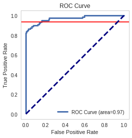
index = numpy.where(numpy.round(false_positive_rate, 2)==0.16)[0][0]
print("True positive rate where false positive rate is 0.16: {0}".format(true_positive_rate[index]))
True positive rate where false positive rate is 0.16: 0.9375
- def true_positive_where_false(model, threshold):
- """get the true-positive value matching the threshold for false-positive
- Args:
- model: the model fit to the data with predict_proba method
- Return:
- float: True Positive rate
System Message: WARNING/2 (<string>, line 466)
Definition list ends without a blank line; unexpected unindent.
"""
y_score_lr = model.predict_proba(X_test)
false_positive_rate, true_positive_rate, _ = roc_curve(y_test, y_score_lr[:, 1])
index = numpy.where(numpy.round(false_positive_rate, 2)==0.16)[0][0]
return true_positive_rate[index]
- def recall_where_precision(model, threshold):
- """return recall where the first precision matches threshold
- Args:
- model: model fit to the data with decision_function
threshold (float): point to find matching recall
- Returns:
- float: recall matching precision threshold
System Message: WARNING/2 (<string>, line 482)
Definition list ends without a blank line; unexpected unindent.
"""
y_scores = model.decision_function(X_test)
precision, recall, thresholds = precision_recall_curve(y_test, y_scores)
return recall[numpy.where(precision==threshold)[0][0]]
- def answer_five():
- model = LogisticRegression()
model.fit(X_train, y_train)
recall_score = recall_where_precision(model, 0.75)
true_positive = true_positive_where_false(model, threshold=0.16)
return (recall_score, true_positive)
answer_five()
parameters = dict(penalty=["l1", "l2"], C=[10**power for power in range(-2, 3)])
model = LogisticRegression()
grid = GridSearchCV(model, parameters, scoring="recall")
grid.fit(X_train, y_train)
grid.cv_results_
len(grid.cv_results_["mean_test_score"])
grid.cv_results_
l1 = [grid.cv_results_["mean_test_score"][index] for index in range(0, len(grid.cv_results_['mean_test_score']), 2)]
l2 = [grid.cv_results_["mean_test_score"][index] for index in range(1, len(grid.cv_results_["mean_test_score"])+ 1, 2)]
l1
l2
- def answer_six():
- parameters = dict(penalty=["l1", "l2"], C=[10**power for power in range(-2, 3)])
model = LogisticRegression()
grid = GridSearchCV(model, parameters, scoring="recall")
grid.fit(X_train, y_train)
l1 = [grid.cv_results_["mean_test_score"][index] for index in range(0, len(grid.cv_results_['mean_test_score']), 2)]
l2 = [grid.cv_results_["mean_test_score"][index] for index in range(1, len(grid.cv_results_["mean_test_score"])+ 1, 2)]
return numpy.array([l1, l2]).T
answer_six()
- def GridSearch_Heatmap(scores):
- get_ipython().magic('matplotlib inline')
import seaborn as sns
import matplotlib.pyplot as plt
plt.figure()
scores = answer_six()
sns.heatmap(scores, xticklabels=['l1','l2'], yticklabels=[0.01, 0.1, 1, 10, 100])
plt.yticks(rotation=0);
- if VERBOSE:
- GridSearch_Heatmap(answer_six())