California Housing Prices
Table of Contents
Introduction
This is an introductory regression problem that uses California housing data from the 1990 census. There's a description of the original data here, but we're using a slightly altered dataset that's on github (and appears to be mirrored on kaggle). The problem here is to create a model that will predict the median housing value for a census block group (called "district" in the dataset) given the other attributes. The original data is also available from sklearn so I'm going to take advantage of that to get the description and do a double-check of the model.
Imports
These are the dependencies for this problem.
# python standard library
import os
import tarfile
import warnings
warnings.filterwarnings("ignore", message="numpy.dtype size changed")
from http import HTTPStatus

# from pypi
import matplotlib
import pandas
import requests
import seaborn
from sklearn.datasets import fetch_california_housing
from tabulate import tabulate
Constants
These are convenience holders for strings and other constants so they don't get scattered all over the place.
class Data:
    source_slug = "../data/california-housing-prices/"
    target_slug = "../data_temp/california-housing-prices/"
    url = "https://github.com/ageron/handson-ml/raw/master/datasets/housing/housing.tgz"
    source = source_slug + "housing.tgz"
    target = target_slug + "housing.csv"
    chunk_size = 128
The Data
We'll grab the data from github, extract it (it's a tgz compressed tarfile), then make a pandas data frame from it. I'll also download the sklearn version.
Downloading the sklearn dataset
sklearn_housing_bunch = fetch_california_housing("~/data/sklearn_datasets/")
Downloading Cal. housing from https://ndownloader.figshare.com/files/5976036 to /home/brunhilde/data/sklearn_datasets/
print(sklearn_housing_bunch.DESCR)
California housing dataset.

The original database is available from StatLib

    http://lib.stat.cmu.edu/datasets/

The data contains 20,640 observations on 9 variables.

This dataset contains the average house value as target variable
and the following input variables (features): average income,
housing average age, average rooms, average bedrooms, population,
average occupation, latitude, and longitude in that order.

References
----------

Pace, R. Kelley and Ronald Barry, Sparse Spatial Autoregressions,
Statistics and Probability Letters, 33 (1997) 291-297.
print(sklearn_housing_bunch.feature_names)
['MedInc', 'HouseAge', 'AveRooms', 'AveBedrms', 'Population', 'AveOccup', 'Latitude', 'Longitude']
Now I'll convert it to a Pandas DataFrame.
sklearn_housing = pandas.DataFrame(sklearn_housing_bunch.data,
				   columns=sklearn_housing_bunch.feature_names)
             MedInc      HouseAge      AveRooms     AveBedrms    Population  \
count  20640.000000  20640.000000  20640.000000  20640.000000  20640.000000
mean       3.870671     28.639486      5.429000      1.096675   1425.476744
std        1.899822     12.585558      2.474173      0.473911   1132.462122
min        0.499900      1.000000      0.846154      0.333333      3.000000
25%        2.563400     18.000000      4.440716      1.006079    787.000000
50%        3.534800     29.000000      5.229129      1.048780   1166.000000
75%        4.743250     37.000000      6.052381      1.099526   1725.000000
max       15.000100     52.000000    141.909091     34.066667  35682.000000

           AveOccup      Latitude     Longitude
count  20640.000000  20640.000000  20640.000000
mean       3.070655     35.631861   -119.569704
std       10.386050      2.135952      2.003532
min        0.692308     32.540000   -124.350000
25%        2.429741     33.930000   -121.800000
50%        2.818116     34.260000   -118.490000
75%        3.282261     37.710000   -118.010000
max     1243.333333     41.950000   -114.310000
Downloading and uncompressing the data
def get_data():
    """Gets the data from github and uncompresses it"""
    if os.path.exists(Data.target):
	return

    os.makedirs(Data.target_slug, exist_ok=True)
    os.makedirs(Data.source_slug, exist_ok=True)
    response = requests.get(Data.url, stream=True)
    assert response.status_code == HTTPStatus.OK
    with open(Data.source, "wb") as writer:
	for chunk in response.iter_content(chunk_size=Data.chunk_size):
	    writer.write(chunk)
    assert os.path.exists(Data.source)
    compressed = tarfile.open(Data.source)
    compressed.extractall(Data.target_slug)
    compressed.close()
    assert os.path.exists(Data.target)
    return
Contents of ../data_temp/california-housing-prices/:
- housing.csv
Building the dataframe
housing = pandas.read_csv(Data.target)
<class 'pandas.core.frame.DataFrame'>
RangeIndex: 20640 entries, 0 to 20639
Data columns (total 10 columns):
longitude             20640 non-null float64
latitude              20640 non-null float64
housing_median_age    20640 non-null float64
total_rooms           20640 non-null float64
total_bedrooms        20433 non-null float64
population            20640 non-null float64
households            20640 non-null float64
median_income         20640 non-null float64
median_house_value    20640 non-null float64
ocean_proximity       20640 non-null object
dtypes: float64(9), object(1)
memory usage: 1.6+ MB
None
Comparison to Sklearn
The dataset seems to differ somewhat from the sklearn description. Instead of total_rooms they have AveRooms, for instance. Is this just a problem of names?
print(sklearn_housing.AveRooms.head())
0 6.984127 1 6.238137 2 8.288136 3 5.817352 4 6.281853 Name: AveRooms, dtype: float64
print(housing.total_rooms.head())
0 880.0 1 7099.0 2 1467.0 3 1274.0 4 1627.0 Name: total_rooms, dtype: float64
So they are different. Let's see if you can get the sklearn values from the original data set.
print((housing.total_rooms/housing.households).head())
0 6.984127 1 6.238137 2 8.288136 3 5.817352 4 6.281853 dtype: float64
It looks like the sklearn values are (in some cases) calculated values derived from the original. It makes sense that they changed some of the things (total number of rooms only makes sense if there is the same number of households in each district, for instance), but it would have been better if they documented the changes they made and why they changed it.
Inspecting the Data
If you look at the total_bedrooms count you'll see that it only has 20,433 non-null values, while the rest of the columns have 20,640 values. These were removed to allow experimenting with missing data. The original dataset that was collected for the census had all the values.
| Column | Has Missing Values |
|---|---|
| longitude | False |
| latitude | False |
| housing_median_age | False |
| total_rooms | False |
| total_bedrooms | True |
| population | False |
| households | False |
| median_income | False |
| median_house_value | False |
| ocean_proximity | False |
It looks like total_bedrooms is the only column where there's missing data.
| Rows | Columns |
|---|---|
| 20640 | 10 |
I'll print the median for each column except the last (since it's non-numeric).
| longitude | latitude | housing_median_age | total_rooms |
|---|---|---|---|
| -118.49 | 34.26 | 29.00 | 2127.00 |
| total_bedrooms | population | households | median_income | median_house_value |
|---|---|---|---|---|
| 435.00 | 1166.00 | 409.00 | 3.53 | 179700.00 |
Here's the description for the ocean_proximity variable
Looking at the median_income you can see that it isn't income in dollars.
| Statistic | Value |
|---|---|
| count | 20640 |
| unique | 5 |
| top | <1H OCEAN |
| freq | 9136 |
It looks like the most common house location is less than an hour from the ocean.
print(
    "{:.2f}".format(
	ocean_proximity_description.loc["freq"]/ocean_proximity_description.loc["count"]))
0.44
Which makes up about forty-four percent of all the houses. Here are all the ocean_proximity values.
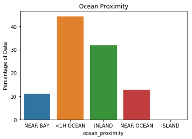
| Proximity | Count | Percentage |
|---|---|---|
| <1H OCEAN | 9136 | 44.2636 |
| INLAND | 6551 | 31.7393 |
| NEAR OCEAN | 2658 | 12.8779 |
| NEAR BAY | 2290 | 11.095 |
| ISLAND | 5 | 0.0242248 |
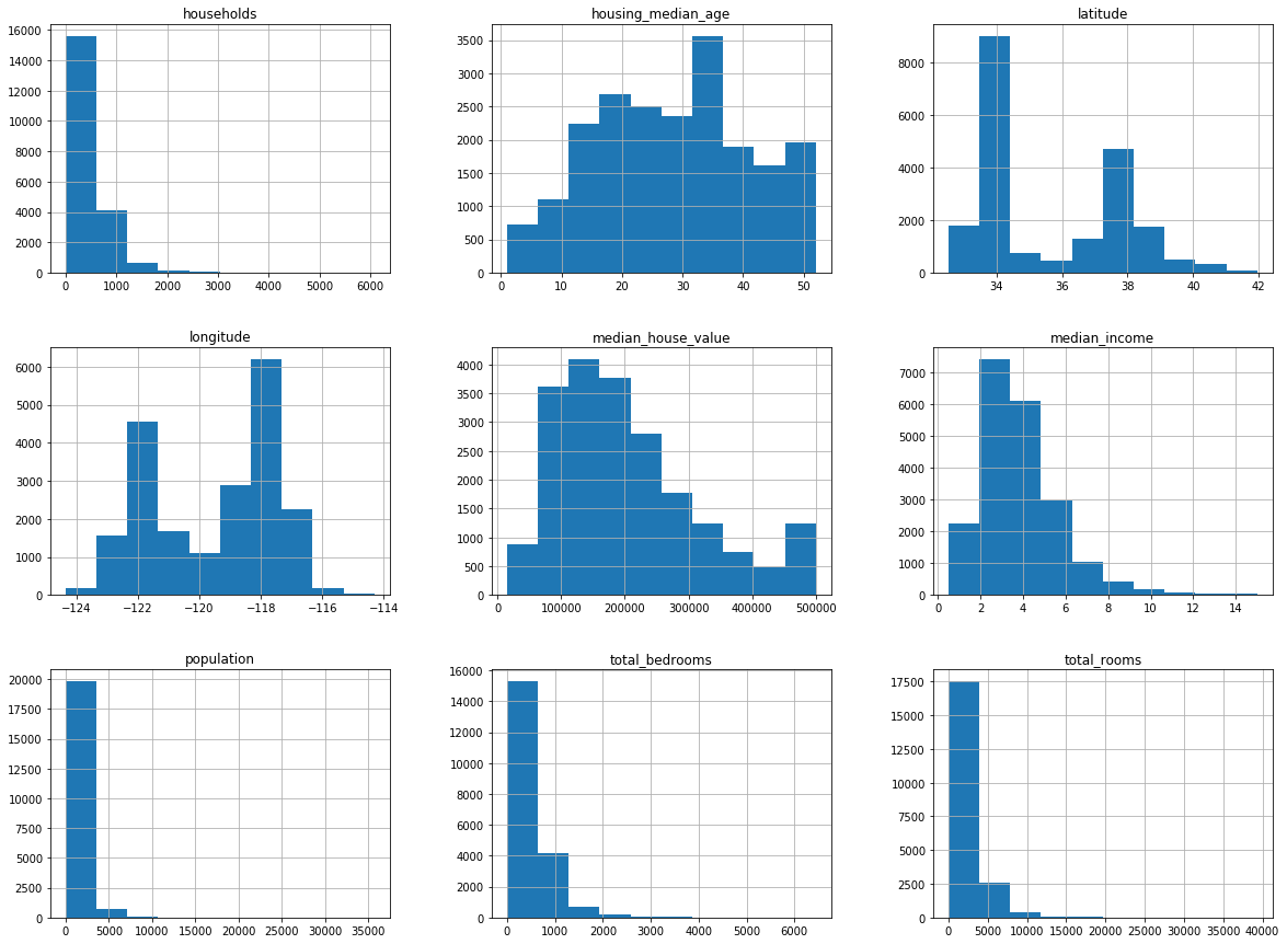
If you look at the median income plot you can see that it goes from 0 to 15. It turns out that the incomes were re-scaled and limited to the 0.5 to 15 range. The median age and value were also capped, possibly affecting our price predictions.
References
- Géron, Aurélien. Hands-on Machine Learning with Scikit-Learn and TensorFlow: Concepts, Tools, and Techniques to Build Intelligent Systems. First edition. Beijing Boston Farnham: O’Reilly, 2017.