Visualizing Max Pooling
Table of Contents
Introduction
This is from Udacity's Deep Learning Repository which supports their Deep Learning Nanodegree.
In this notebook, we will visualize the output of a maxpooling layer in a CNN.
A convolutional layer + activation function, followed by a pooling layer, and a linear layer (to create a desired output size) make up the basic layers of a CNN.
Set Up
Imports
PyPi
from dotenv import load_dotenv
import cv2
import matplotlib.pyplot as pyplot
import numpy
import seaborn
import torch
import torch.nn as nn
import torch.nn.functional as F
This Project
from neurotic.tangles.data_paths import DataPathTwo
Plotting
get_ipython().run_line_magic('matplotlib', 'inline')
seaborn.set(style="whitegrid",
            rc={"axes.grid": False,
                "font.family": ["sans-serif"],
                "font.sans-serif": ["Latin Modern Sans", "Lato"],
                "figure.figsize": (14, 12)},
            font_scale=3)
Load the Data
load_dotenv()
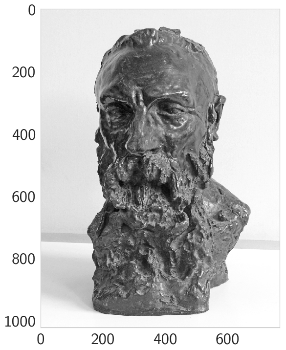
path = DataPathTwo("rodin.jpg", "CNN")
print(path.from_folder)
assert path.from_folder.is_file()
/home/brunhilde/datasets/cnn/rodin.jpg
bgr_img = cv2.imread(str(path.from_folder))
Convert To Grayscale
gray_img = cv2.cvtColor(bgr_img, cv2.COLOR_BGR2GRAY)
Normalize: Rescale Entries To Lie In [0,1]
gray_img = gray_img.astype("float32")/255
image = pyplot.imshow(gray_img, cmap='gray')
Define and visualize the filters
filter_vals = numpy.array([[-1, -1, -1],
                           [-1, 8, -1],
                           [-1, -1, -1]])
print('Filter shape: ', filter_vals.shape)
Filter shape: (3, 3)
Defining four different filters,
All of these are linear combinations of the filter_vals defined above
filter_1 = filter_vals
filter_2 = -filter_1
filter_3 = filter_1.T
filter_4 = -filter_3
filters = numpy.array([filter_1, filter_2, filter_3, filter_4])
print('Filter 1: \n', filter_4)
Filter 1:
 [[ 1  1  1]
 [ 1 -8  1]
 [ 1  1  1]]
Define convolutional and pooling layers
You've seen how to define a convolutional layer, next is a Pooling Layer.
In the next cell, we initialize a convolutional layer so that it contains all the created filters. Then add a maxpooling layer, documented here, with a kernel size of (2x2) so you can see that the image resolution has been reduced after this step.
A maxpooling layer reduces the x-y size of an input and only keeps the most active pixel values. Below is an example of a 2x2 pooling kernel, with a stride of 2, appied to a small patch of grayscale pixel values; reducing the x-y size of the patch by a factor of 2. Only the maximum pixel values in 2x2 remain in the new, pooled output.
Define a neural network with a convolutional layer with four filters and a pooling layer of size (2, 2).
The Model
class Net(nn.Module):
    """A convolutional neural network to process 4 filters

    Args:
     weight: matrix of filters
    """
    def __init__(self, weight: numpy.ndarray) -> None:
        super(Net, self).__init__()
        # initializes the weights of the convolutional layer to be the weights of the 4 defined filters
        k_height, k_width = weight.shape[2:]
        # assumes there are 4 grayscale filters
        self.conv = nn.Conv2d(1, 4, kernel_size=(k_height, k_width), bias=False)
        self.conv.weight = torch.nn.Parameter(weight)
        # define a pooling layer
        self.pool = nn.MaxPool2d(2, 2)
        return

    def forward(self, x: torch.Tensor):
        """calculates the output of a convolutional layer

        Args:
         x: image to process

        Returns:
         layers: convolutional, activated, and pooled layers
        """
        conv_x = self.conv(x)
        activated_x = F.relu(conv_x)

        # applies pooling layer
        pooled_x = self.pool(activated_x)

        # returns all layers
        return conv_x, activated_x, pooled_x
instantiate the model and set the weights
weight = torch.from_numpy(filters).unsqueeze(1).type(torch.FloatTensor)
model = Net(weight)
print(model)
Net(
  (conv): Conv2d(1, 4, kernel_size=(3, 3), stride=(1, 1), bias=False)
  (pool): MaxPool2d(kernel_size=2, stride=2, padding=0, dilation=1, ceil_mode=False)
)
Visualize the output of each filter
First, we'll define a helper function, viz_layer that takes in a specific layer and number of filters (optional argument), and displays the output of that layer once an image has been passed through.
def viz_layer(layer, n_filters= 4):
    fig = pyplot.figure(figsize=(20, 20))

    for i in range(n_filters):
        ax = fig.add_subplot(1, n_filters, i+1)
        # grab layer outputs
        ax.imshow(numpy.squeeze(layer[0,i].data.numpy()), cmap='gray')
        ax.set_title('Output %s' % str(i+1))
    return
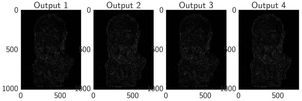
Let's look at the output of a convolutional layer after a ReLu activation function is applied.
ReLu activation
A ReLu function turns all negative pixel values in 0's (black). See the equation pictured below for input pixel values, x.
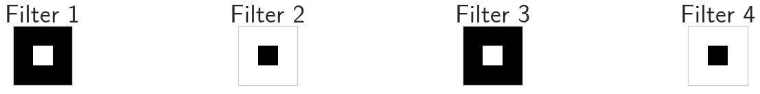
Visualize All the Filters
fig = pyplot.figure(figsize=(12, 6))
fig.subplots_adjust(left=0, right=1.5, bottom=0.8, top=1, hspace=0.05, wspace=0.05)
for i in range(4):
    ax = fig.add_subplot(1, 4, i+1, xticks=[], yticks=[])
    ax.imshow(filters[i], cmap='gray')
    ax.set_title('Filter %s' % str(i+1))
convert the image into an input Tensor
gray_img_tensor = torch.from_numpy(gray_img).unsqueeze(0).unsqueeze(1)
get all the layers
conv_layer, activated_layer, pooled_layer = model(gray_img_tensor)
visualize the output of the activated conv layer
viz_layer(activated_layer)
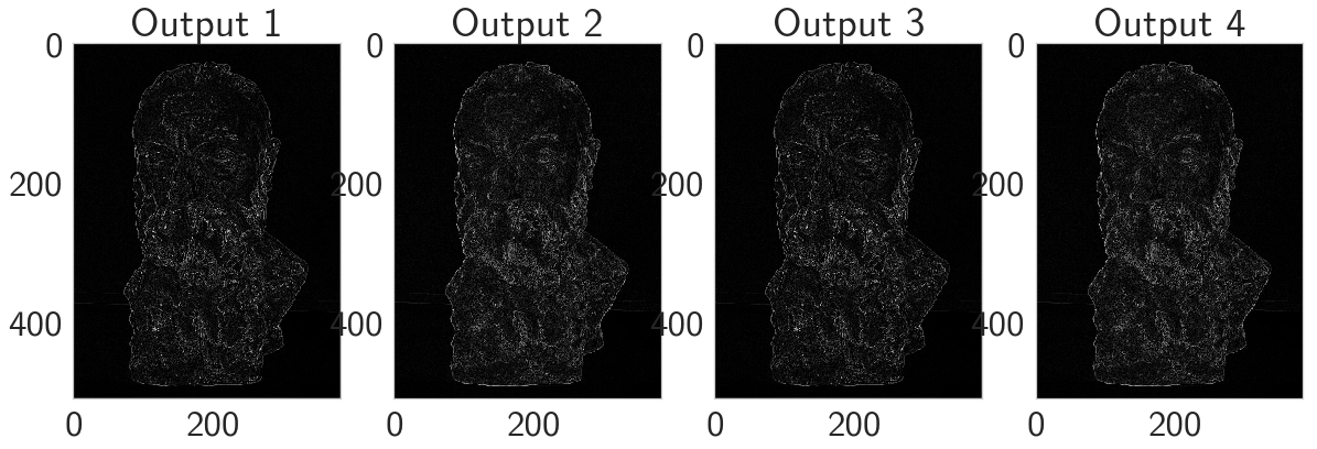
Visualize the output of the pooling layer
Then, take a look at the output of a pooling layer. The pooling layer takes as input the feature maps pictured above and reduces the dimensionality of those maps, by some pooling factor, by constructing a new, smaller image of only the maximum (brightest) values in a given kernel area.
Take a look at the values on the x, y axes to see how the image has changed size.
viz_layer(pooled_layer)