Visualizing Convolving
Table of Contents
Introduction
This is from Udacity's Deep Learning Repository which supports their Deep Learning Nanodegree.
In this notebook, we visualize four filtered outputs (a.k.a. activation maps) of a convolutional layer.
In this example, we are defining four filters that are applied to an input image by initializing the weights of a convolutional layer, but a trained CNN will learn the values of these weights.
Imports
PyPi
from dotenv import load_dotenv
import cv2
import matplotlib.pyplot as pyplot
import numpy
import seaborn
import torch
import torch.nn as nn
import torch.nn.functional as F
This Project
from neurotic.tangles.data_paths import DataPathTwo
Set Up Plotting
get_ipython().run_line_magic('matplotlib', 'inline')
seaborn.set(style="whitegrid",
            rc={"axes.grid": False,
                "font.family": ["sans-serif"],
                "font.sans-serif": ["Latin Modern Sans", "Lato"],
                "figure.figsize": (14, 12)},
            font_scale=3)
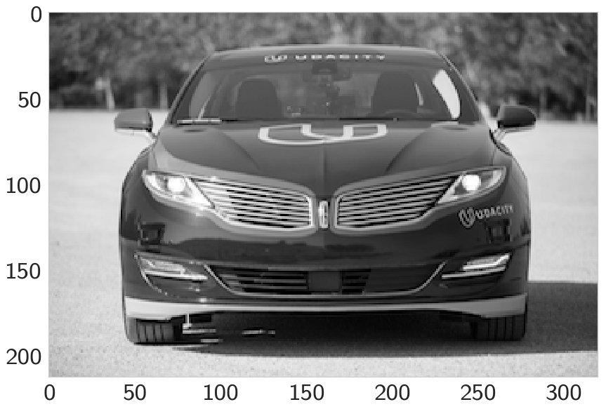
The Image
load_dotenv()
path = DataPathTwo("udacity_sdc.png", folder_key="CNN")
Load the Image
bgr_img = cv2.imread(str(path.from_folder))
Convert It To Grayscale
gray_img = cv2.cvtColor(bgr_img, cv2.COLOR_BGR2GRAY)
Normalize By Rescaling the Entries To Lie In [0,1]
gray_img = gray_img.astype("float32")/255
Plot the Image
image = pyplot.imshow(gray_img, cmap='gray')

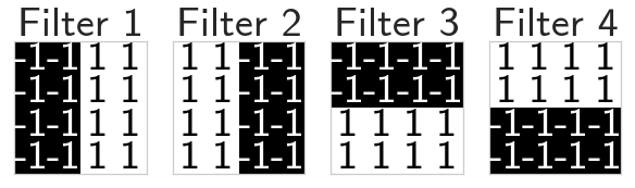
Define and Visualize the Filters
filter_vals = numpy.array([[-1, -1, 1, 1], [-1, -1, 1, 1], [-1, -1, 1, 1], [-1, -1, 1, 1]])

print('Filter shape: ', filter_vals.shape)
Filter shape: (4, 4)
Defining four different filters,
All of these are linear combinations of the filter_vals defined above.
filter_1 = filter_vals
filter_2 = -filter_1
filter_3 = filter_1.T
filter_4 = -filter_3
filters = numpy.array([filter_1, filter_2, filter_3, filter_4])
Here's what filter_1 has.
print('Filter 1: \n', filter_1)
Filter 1:
 [[-1 -1  1  1]
 [-1 -1  1  1]
 [-1 -1  1  1]
 [-1 -1  1  1]]
Visualize All Four Filters
fig = pyplot.figure(figsize=(10, 5))
for i in range(4):
    ax = fig.add_subplot(1, 4, i+1, xticks=[], yticks=[])
    ax.imshow(filters[i], cmap='gray')
    ax.set_title('Filter %s' % str(i+1))
    width, height = filters[i].shape
    for x in range(width):
        for y in range(height):
            ax.annotate(str(filters[i][x][y]), xy=(y,x),
                        horizontalalignment='center',
                        verticalalignment='center',
                        color='white' if filters[i][x][y]<0 else 'black')
Define a convolutional layer
The various layers that make up any neural network are documented, here. For a convolutional neural network, we'll start by defining a:
- Convolutional Layer
Initialize a single convolutional layer so that it contains all your created filters. Note that you are not training this network; you are initializing the weights in a convolutional layer so that you can visualize what happens after a forward pass through this network!
__init__ and forward
To define a neural network in PyTorch, you define the layers of a model in the __init__ method and define the forward behavior of a network that applyies those initialized layers to an input (x) in the forward method. In PyTorch we convert all inputs into the Tensor datatype, which is similar to a list data type in Python.
Below is a class called Net that has a convolutional layer that can contain four 3x3 grayscale filters.
This will be a neural network with a single convolutional layer with four filters.
class Net(nn.Module):
    """CNN To apply 4 filters

    initializes the weights of the convolutional layer to be the
    weights of the 4 defined filters

    Args:
     weights: array with the four filters
    """
    def __init__(self, weight):
        super(Net, self).__init__()
        k_height, k_width = weight.shape[2:]
        # assumes there are 4 grayscale filters
        self.conv = nn.Conv2d(1, 4, kernel_size=(k_height, k_width), bias=False)
        self.conv.weight = torch.nn.Parameter(weight)
        return

    def forward(self, x):
        """calculates the output of a convolutional layer
        pre- and post-activation

        Args:
         x: the image to apply the convolution to

        Returns:
         tuple: convolution output, relu output
        """
        conv_x = self.conv(x)
        activated_x = F.relu(conv_x)

        # returns both layers
        return conv_x, activated_x
Instantiate the Model and Set the Weights
weight = torch.from_numpy(filters).unsqueeze(1).type(torch.FloatTensor)
model = Net(weight)
print(model)
Net(
  (conv): Conv2d(1, 4, kernel_size=(4, 4), stride=(1, 1), bias=False)
)
Visualize the output of each filter
First, we'll define a helper function, viz_layer that takes in a specific layer and number of filters (optional argument), and displays the output of that layer once an image has been passed through.
def viz_layer(layer, n_filters= 4):
    fig = pyplot.figure(figsize=(20, 20))

    for i in range(n_filters):
        ax = fig.add_subplot(1, n_filters, i+1, xticks=[], yticks=[])
        # grab layer outputs
        ax.imshow(numpy.squeeze(layer[0,i].data.numpy()), cmap='gray')
        ax.set_title('Output %s' % str(i+1))
    return
Let's look at the output of a convolutional layer, before and after a ReLu activation function is applied. First, here's our original image again.
image = pyplot.imshow(gray_img, cmap='gray')
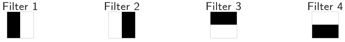
visualize all filters
fig = pyplot.figure(figsize=(12, 6))
fig.subplots_adjust(left=0, right=1.5, bottom=0.8, top=1, hspace=0.05, wspace=0.05)
for i in range(4):
    ax = fig.add_subplot(1, 4, i+1, xticks=[], yticks=[])
    ax.imshow(filters[i], cmap='gray')
    ax.set_title('Filter %s' % str(i+1))
Convert The Image Into An Input Tensor
gray_img_tensor = torch.from_numpy(gray_img).unsqueeze(0).unsqueeze(1)
Get The Convolutional Layer (Pre and Post Activation)
conv_layer, activated_layer = model(gray_img_tensor)
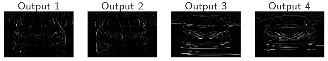
Visualize the Output of a Convolutional Layer
viz_layer(conv_layer)
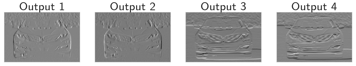
Sort of gives it a bas-relief look.
ReLu activation
In this model, we've used an activation function that scales the output of the convolutional layer. We've chose a ReLu function to do this, and this function simply turns all negative pixel values to 0's (black). See the equation pictured below for input pixel values, x.
Visualize the output of an activated conv layer after a ReLu is applied.
viz_layer(activated_layer)