Weight Initialization
Table of Contents
- Introduction
- Initial Weights and Observing Training Loss
- Dataset and Model
- Import Libraries and Load the Data
- Visualize Some Training Data
- Define the Model Architecture
- Initialize Weights
- Compare Model Behavior
- General rule for setting weights
- Normal Distribution
- Automatic Initialization
- evaluate the behavior using helpers
Introduction
In this lesson, you'll learn how to find good initial weights for a neural network. Weight initialization happens once, when a model is created and before it trains. Having good initial weights can place the neural network close to the optimal solution. This allows the neural network to come to the best solution quicker.
Initial Weights and Observing Training Loss
To see how different weights perform, we'll test on the same dataset and neural network. That way, we know that any changes in model behavior are due to the weights and not any changing data or model structure. We'll instantiate at least two of the same models, with different initial weights and see how the training loss decreases over time.
Sometimes the differences in training loss, over time, will be large and other times, certain weights offer only small improvements.
Dataset and Model
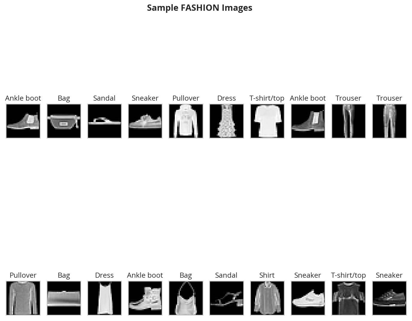
We'll train an MLP to classify images from the Fashion-MNIST database to demonstrate the effect of different initial weights. As a reminder, the FashionMNIST dataset contains images of clothing types; classes = ['T-shirt/top', 'Trouser', 'Pullover', 'Dress', 'Coat', 'Sandal', 'Shirt', 'Sneaker', 'Bag', 'Ankle boot']. The images are normalized so that their pixel values are in a range [0.0 - 1.0). Run the cell below to download and load the dataset.
Import Libraries and Load the Data
Imports
# python
from functools import partial
from typing import Collection, Tuple
# from pypi
from dotenv import load_dotenv
from sklearn.model_selection import train_test_split
from torch.utils.data.sampler import SubsetRandomSampler
from torchvision import datasets
import matplotlib.pyplot as pyplot
import numpy
import seaborn
import torch
import torch.nn as nn
import torch.nn.functional as F
import torchvision.transforms as transforms

# udacity
import nano.helpers as helpers

# this project
from neurotic.tangles.data_paths import DataPathTwo
Load the Data
# number of subprocesses to use for data loading
subprocesses = 0
# how many samples per batch to load
batch_size = 100
# percentage of training set to use as validation
VALIDATION_FRACTION = 0.2
Convert the data to a torch.FloatTensor.
transform = transforms.ToTensor()
load_dotenv()
path = DataPathTwo(folder_key="FASHION")
print(path.folder)
/home/brunhilde/datasets/FASHION
Choose the training and test datasets.
train_data = datasets.FashionMNIST(root=path.folder, train=True,
                                   download=True, transform=transform)
test_data = datasets.FashionMNIST(root=path.folder, train=False,
                                  download=True, transform=transform)
Downloading http://fashion-mnist.s3-website.eu-central-1.amazonaws.com/train-images-idx3-ubyte.gz
Downloading http://fashion-mnist.s3-website.eu-central-1.amazonaws.com/train-labels-idx1-ubyte.gz
Downloading http://fashion-mnist.s3-website.eu-central-1.amazonaws.com/t10k-images-idx3-ubyte.gz
Downloading http://fashion-mnist.s3-website.eu-central-1.amazonaws.com/t10k-labels-idx1-ubyte.gz
Processing...
Done!
Obtain training indices that will be used for validation.
indices = list(range(len(train_data)))
train_idx, valid_idx = train_test_split(
    indices,
    test_size=VALIDATION_FRACTION)
Define samplers for obtaining training and validation batches.
train_sampler = SubsetRandomSampler(train_idx)
valid_sampler = SubsetRandomSampler(valid_idx)
Prepare data loaders (combine dataset and sampler).
train_loader = torch.utils.data.DataLoader(train_data, batch_size=batch_size,
                                           sampler=train_sampler, num_workers=subprocesses)
valid_loader = torch.utils.data.DataLoader(train_data, batch_size=batch_size,
                                           sampler=valid_sampler, num_workers=subprocesses)
test_loader = torch.utils.data.DataLoader(test_data, batch_size=batch_size,
                                          num_workers=subprocesses)
classes = ['T-shirt/top', 'Trouser', 'Pullover', 'Dress', 'Coat',
    'Sandal', 'Shirt', 'Sneaker', 'Bag', 'Ankle boot']
Visualize Some Training Data
get_ipython().run_line_magic('matplotlib', 'inline')
get_ipython().run_line_magic('config', "InlineBackend.figure_format = 'retina'")
seaborn.set(style="whitegrid",
            rc={"axes.grid": False,
                "font.family": ["sans-serif"],
                "font.sans-serif": ["Open Sans", "Latin Modern Sans", "Lato"],
                "figure.figsize": (10, 8)},
            font_scale=1)
Obtain one batch of training images.
dataiter = iter(train_loader)
images, labels = dataiter.next()
images = images.numpy()
Plot the images in the batch, along with the corresponding labels.
fig = pyplot.figure(figsize=(12, 10))
fig.suptitle("Sample FASHION Images", weight="bold")
for idx in np.arange(20):
    ax = fig.add_subplot(2, 20/2, idx+1, xticks=[], yticks=[])
    ax.imshow(np.squeeze(images[idx]), cmap='gray')
    ax.set_title(classes[labels[idx]])
Define the Model Architecture
We've defined the MLP that we'll use for classifying the dataset.
Neural Network
- A 3 layer MLP with hidden dimensions of 256 and 128.
- This MLP accepts a flattened image (784-value long vector) as input and produces 10 class scores as output.
We'll test the effect of different initial weights on this 3 layer neural network with ReLU activations and an Adam optimizer. The lessons you learn apply to other neural networks, including different activations and optimizers.
Initialize Weights
Let's start looking at some initial weights.
All Zeros or Ones
If you follow the principle of Occam's razor, you might think setting all the weights to 0 or 1 would be the best solution. This is not the case.
With every weight the same, all the neurons at each layer are producing the same output. This makes it hard to decide which weights to adjust.
Let's compare the loss with all ones and all zero weights by defining two models with those constant weights.
Below, we are using PyTorch's nn.init to initialize each Linear layer with a constant weight. The init library provides a number of weight initialization functions that give you the ability to initialize the weights of each layer according to layer type.
In the case below, we look at every layer/module in our model. If it is a Linear layer (as all three layers are for this MLP), then we initialize those layer weights to be a constant_weight with bias=0 using the following code:
if isinstance(m, nn.Linear):
    nn.init.constant_(m.weight, constant_weight)
    nn.init.constant_(m.bias, 0)
The constant_weight is a value that you can pass in when you instantiate the model.
Define the NN architecture
class Net(nn.Module):
    def __init__(self, hidden_1=256, hidden_2=128, constant_weight=None):
        super(Net, self).__init__()
        # linear layer (784 -> hidden_1)
        self.fc1 = nn.Linear(28 * 28, hidden_1)
        # linear layer (hidden_1 -> hidden_2)
        self.fc2 = nn.Linear(hidden_1, hidden_2)
        # linear layer (hidden_2 -> 10)
        self.fc3 = nn.Linear(hidden_2, 10)
        # dropout layer (p=0.2)
        self.dropout = nn.Dropout(0.2)

        # initialize the weights to a specified, constant value
        if(constant_weight is not None):
            for m in self.modules():
                if isinstance(m, nn.Linear):
                    nn.init.constant_(m.weight, constant_weight)
                    nn.init.constant_(m.bias, 0)


    def forward(self, x):
        # flatten image input
        x = x.view(-1, 28 * 28)
        # add hidden layer, with relu activation function
        x = F.relu(self.fc1(x))
        # add dropout layer
        x = self.dropout(x)
        # add hidden layer, with relu activation function
        x = F.relu(self.fc2(x))
        # add dropout layer
        x = self.dropout(x)
        # add output layer
        x = self.fc3(x)
        return x
Compare Model Behavior
Below, we are using helpers.compare_init_weights to compare the training and validation loss for the two models we defined above, model_0 and model_1. This function takes in a list of models (each with different initial weights), the name of the plot to produce, and the training and validation dataset loaders. For each given model, it will plot the training loss for the first 100 batches and print out the validation accuracy after 2 training epochs. Note: if you've used a small batch_size, you may want to increase the number of epochs here to better compare how models behave after seeing a few hundred images.
We plot the loss over the first 100 batches to better judge which model weights performed better at the start of training. I recommend that you take a look at the code in helpers.py to look at the details behind how the models are trained, validated, and compared.
Run the cell below to see the difference between weights of all zeros against all ones.
Initialize two NN's with 0 and 1 constant weights.
model_0 = Net(constant_weight=0)
model_1 = Net(constant_weight=1)
Put them in list form to compare.
model_list = [(model_0, 'All Zeros'),
              (model_1, 'All Ones')]
ModelLabel = Tuple[nn.Module, str]
ModelLabels = Collection[ModelLabel]
def plot_models(title:str, models_labels:ModelLabels):
    """Plots the models

    Args:
     title: the title for the plots
     models_labels: collections of model, plot-label tuples
    """
    figure, axe = pyplot.subplots()
    figure.suptitle(title, weight="bold")
    axe.set_xlabel("Batches")
    axe.set_ylabel("Loss")

    for model, label in models_labels:
        loss, validation_accuracy = helpers._get_loss_acc(model, train_loader, valid_loader)
        axe.plot(loss[:100], label=label)
    legend = axe.legend()
    return
Plot the loss over the first 100 batches.
plot_models("All Zeros vs All Ones",
            ((model_0, "All Zeros"),
             (model_1, "All ones")))
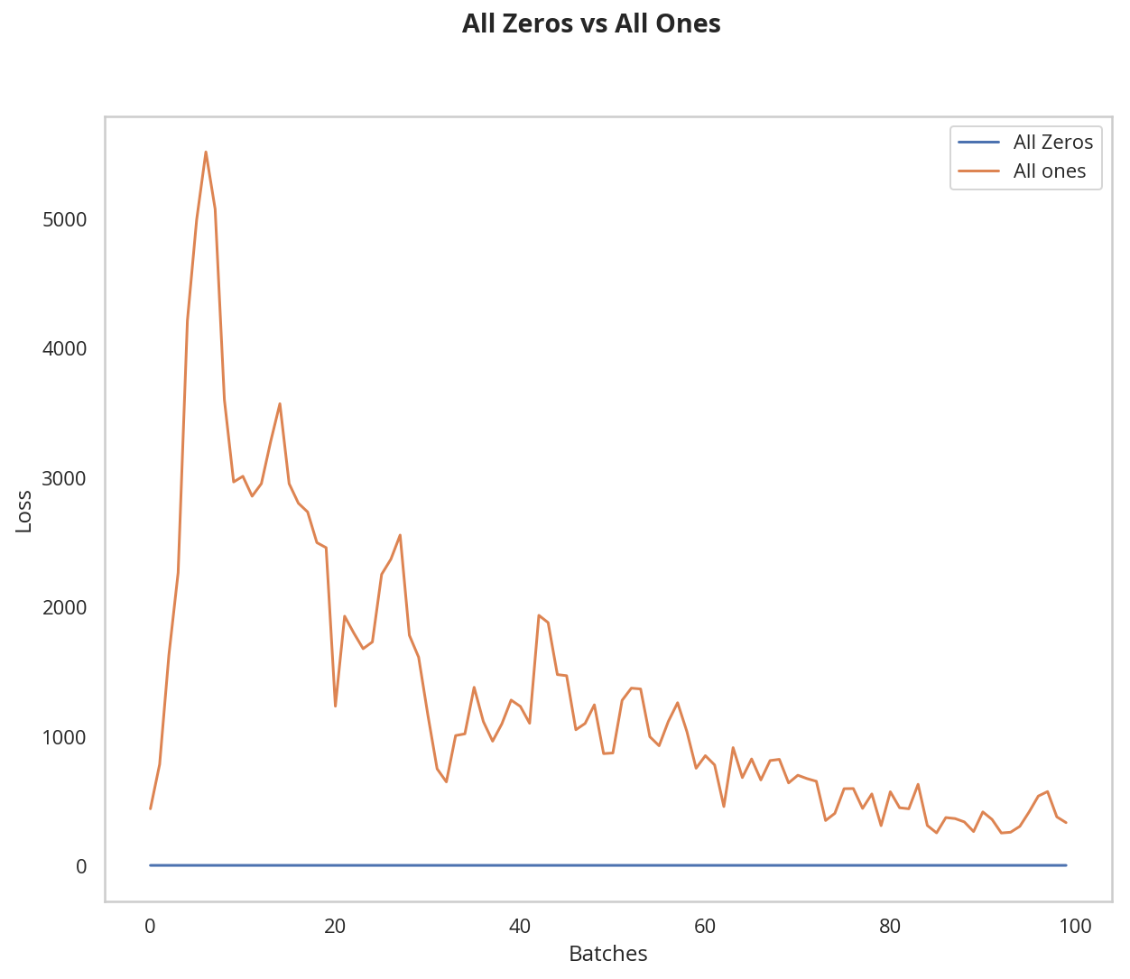
After 2 Epochs:
Validation Accuracy
    9.475% -- All Zeros
   10.175% -- All Ones
Training Loss
    2.304  -- All Zeros
  1914.703  -- All Ones
As you can see the accuracy is close to guessing for both zeros and ones, around 10%.
The neural network is having a hard time determining which weights need to be changed, since the neurons have the same output for each layer. To avoid neurons with the same output, let's use unique weights. We can also randomly select these weights to avoid being stuck in a local minimum for each run.
A good solution for getting these random weights is to sample from a uniform distribution.
Uniform Distribution
A uniform distribution has the equal probability of picking any number from a set of numbers. We'll be picking from a continuous distribution, so the chance of picking the same number is low. We'll use NumPy's np.random.uniform function to pick random numbers from a uniform distribution.
np.random_uniform(low=0.0, high=1.0, size=None)
Outputs random values from a uniform distribution.
The generated values follow a uniform distribution in the range [low, high). The lower bound minval is included in the range, while the upper bound maxval is excluded.
- low: The lower bound on the range of random values to generate. Defaults to 0.
- high: The upper bound on the range of random values to generate. Defaults to 1.
- size: An int or tuple of ints that specify the shape of the output array.
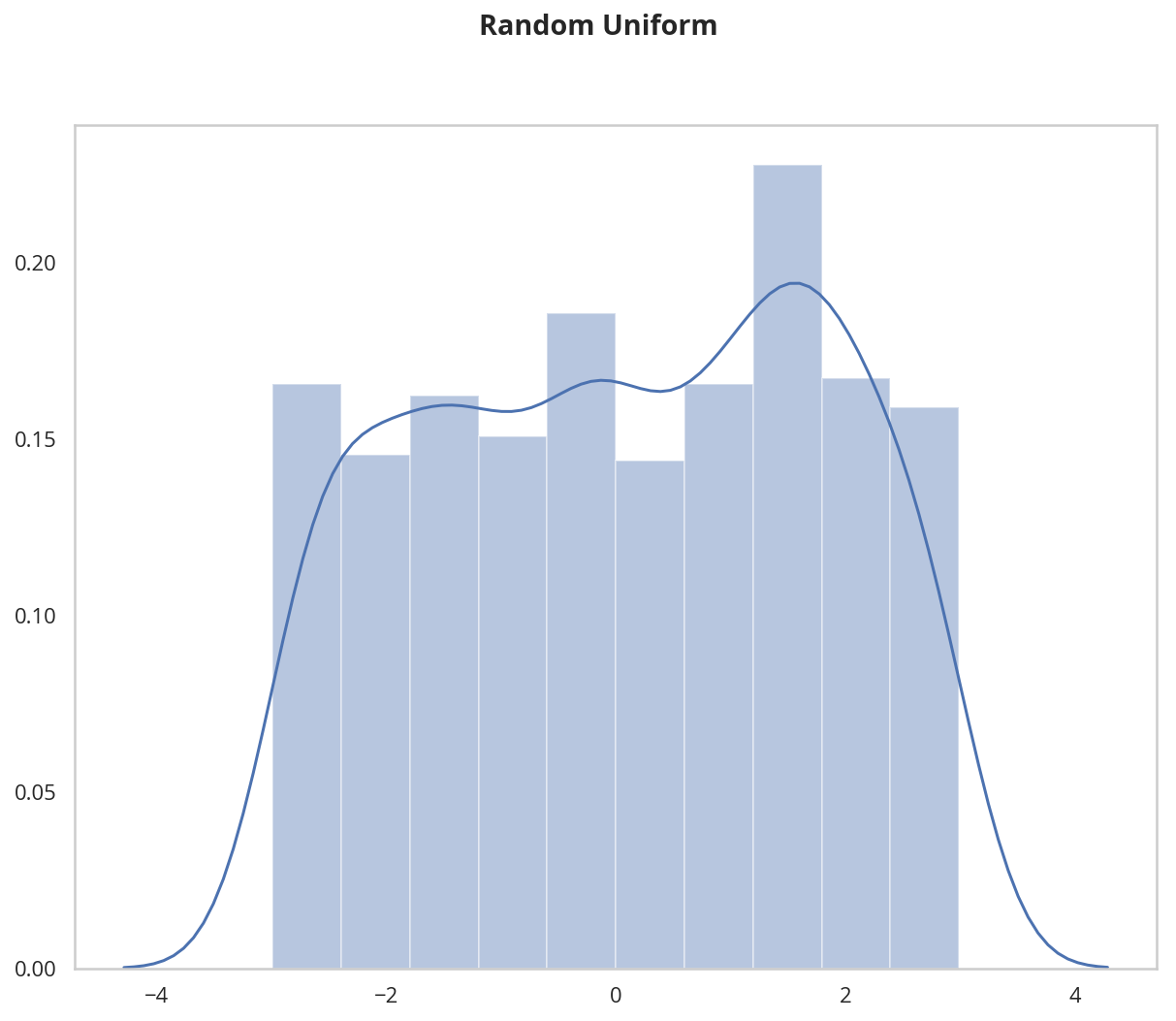
We can visualize the uniform distribution by using a histogram. Let's map the values from np.random_uniform(-3, 3, [1000]) to a histogram using the helper.hist_dist function. This will be 1000 random float values from -3 to 3, excluding the value 3.
figure, axe = pyplot.subplots()
figure.suptitle("Random Uniform", weight="bold")
data = numpy.random.uniform(-3, 3, [1000])
grid = seaborn.distplot(data)
#helpers.hist_dist('Random Uniform (low=-3, high=3)', )
Now that you understand the uniform function, let's use PyTorch's nn.init to apply it to a model's initial weights.
Uniform Initialization, Baseline
Let's see how well the neural network trains using a uniform weight initialization, where low=0.0 and high=1.0. Below, I'll show you another way (besides in the Net class code) to initialize the weights of a network. To define weights outside of the model definition, you can:
- Define a function that assigns weights by the type of network layer, then
- Apply those weights to an initialized model using
model.apply(fn), which applies a function to each model layer.
This time, we'll use weight.data.uniform_ to initialize the weights of our model, directly.
def weights_init_uniform(m: nn.Module, start=0.0, stop=1.0) -> None:
    """takes in a module and applies the specified weight initialization

    Args:
     m: A model instance
    """
    classname = m.__class__.__name__
    # for every Linear layer in a model..
    if classname.startswith('Linear'):
        # apply a uniform distribution to the weights and a bias=0
        m.weight.data.uniform_(start, stop)
        m.bias.data.fill_(0)
    return
Create A New Model With These Weights
Evaluate Behavior
model_uniform = Net()
model_uniform.apply(weights_init_uniform)
plot_models("Uniform Baseline", ((model_uniform, "UNIFORM WEIGHTS"),))
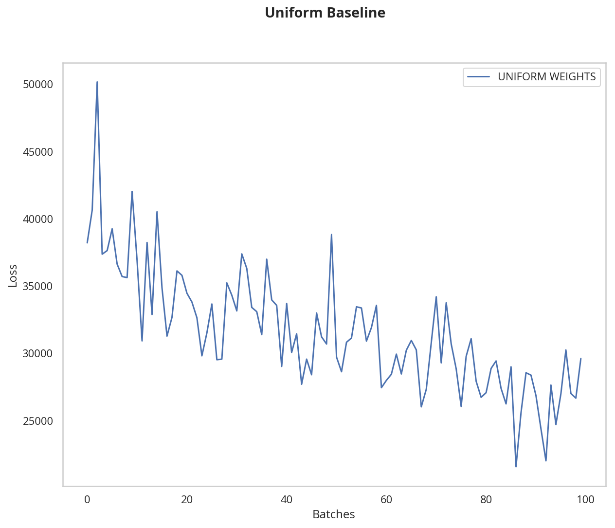
The loss graph is showing the neural network is learning, which it didn't with all zeros or all ones. We're headed in the right direction!
General rule for setting weights
The general rule for setting the weights in a neural network is to set them to be close to zero without being too small. A good practice is to start your weights in the range of \([-y, y]\) where \(y=1/\sqrt{n}\) (\(n\) is the number of inputs to a given neuron).
Let's see if this holds true; let's create a baseline to compare with and center our uniform range over zero by shifting it over by 0.5. This will give us the range [-0.5, 0.5).
weights_init_uniform_center = partial(weights_init_uniform, -0.5, 0.5)
create a new model with these weights
model_centered = Net()
model_centered.apply(weights_init_uniform_center)
Now let's create a distribution and model that uses the general rule for weight initialization; using the range \([-y, y]\), where \(y=1/\sqrt{n}\) .
And finally, we'll compare the two models.
def weights_init_uniform_rule(m: nn.Module) -> None:
    """takes in a module and applies the specified weight initialization

    Args:
     m: Model instance
    """
    classname = m.__class__.__name__
    # for every Linear layer in a model..
    if classname.find('Linear') != -1:
        # get the number of the inputs
        n = m.in_features
        y = 1.0/numpy.sqrt(n)
        m.weight.data.uniform_(-y, y)
        m.bias.data.fill_(0)
    return
model_rule = Net()
model_rule.apply(weights_init_uniform_rule)
plot_models("Uniform Centered vs General Rule", (
    (model_centered, 'Centered Weights [-0.5, 0.5)'),
    (model_rule, 'General Rule [-y, y)'),
))
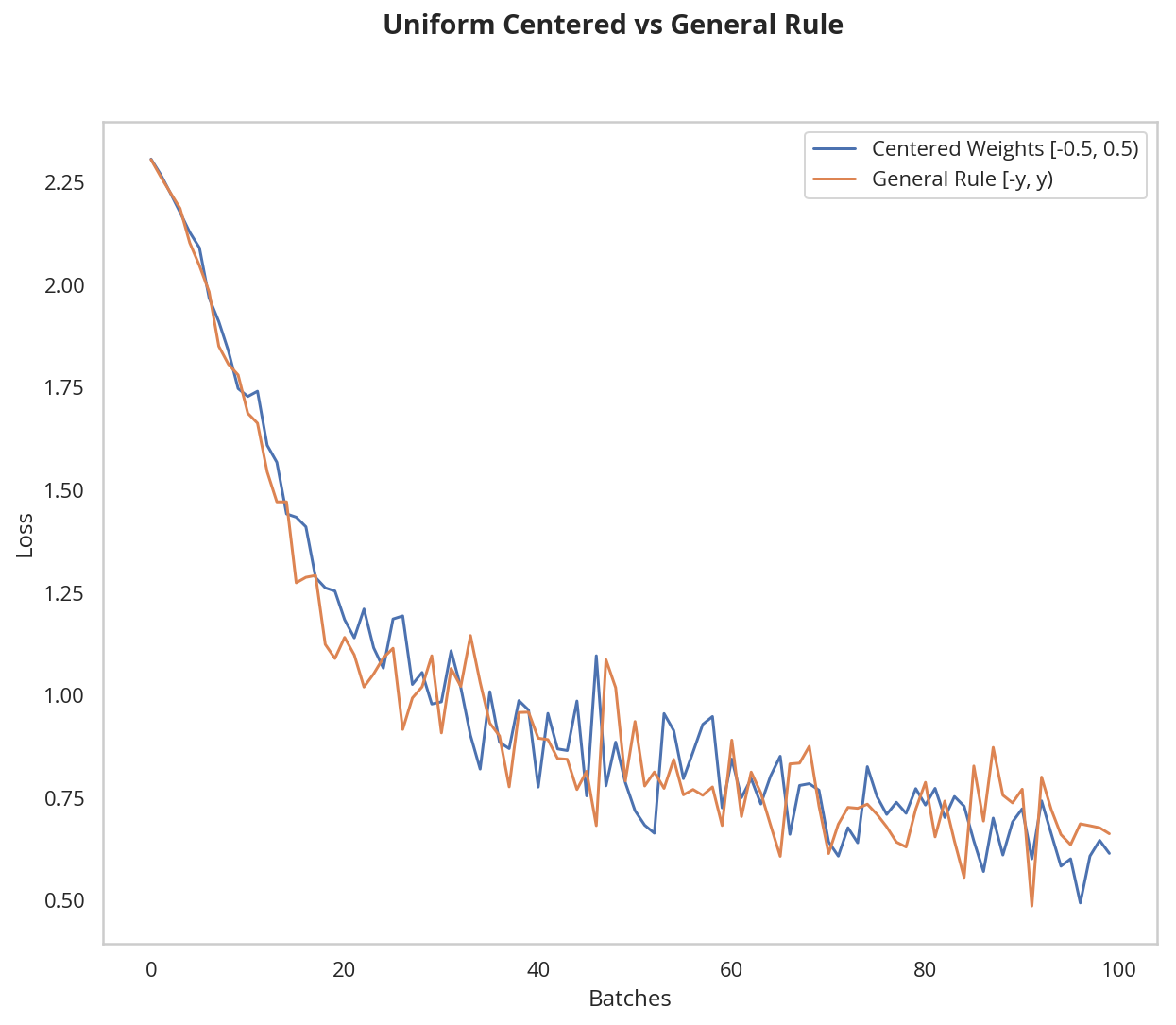 This behavior is really promising! Not only is the loss decreasing, but it seems to do so very quickly for our uniform weights that follow the general rule; after only two epochs we get a fairly high validation accuracy and this should give you some intuition for why starting out with the right initial weights can really help your training process!
Since the uniform distribution has the same chance to pick any value in a range, what if we used a distribution that had a higher chance of picking numbers closer to 0? Let's look at the normal distribution.
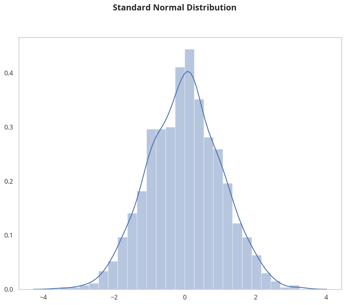
Normal Distribution
Unlike the uniform distribution, the normal distribution has a higher likelihood of picking number close to it's mean. To visualize it, let's plot values from NumPy's np.random.normal function to a histogram.
np.random.normal(loc=0.0, scale=1.0, size=None)
Outputs random values from a normal distribution.
- loc: The mean of the normal distribution.
- scale: The standard deviation of the normal distribution.
- shape: The shape of the output array.
figure, axe = pyplot.subplots()
figure.suptitle("Standard Normal Distribution", weight="bold")
grid = seaborn.distplot(numpy.random.normal(size=[1000]))
Let's compare the normal distribution against the previous, rule-based, uniform distribution.
The normal distribution should have a mean of 0 and a standard deviation of \(y=1/\sqrt{n}\)
def weights_init_normal(m: nn.Module) -> None:
    '''Takes in a module and initializes all linear layers with weight
       values taken from a normal distribution.'''

    classname = m.__class__.__name__
    if classname.startswith("Linear"):
        m.weight.data.normal_(mean=0, std=1/numpy.sqrt(m.in_features))
        m.bias.data.fill_(0)
    return
create a new model with the rule-based, uniform weights
model_uniform_rule = Net()
model_uniform_rule.apply(weights_init_uniform_rule)
create a new model with the rule-based, NORMAL weights
model_normal_rule = Net()
model_normal_rule.apply(weights_init_normal)
compare the two models
plot_models('Uniform vs Normal',
            ((model_uniform_rule, 'Uniform Rule [-y, y)'),
             (model_normal_rule, 'Normal Distribution')))
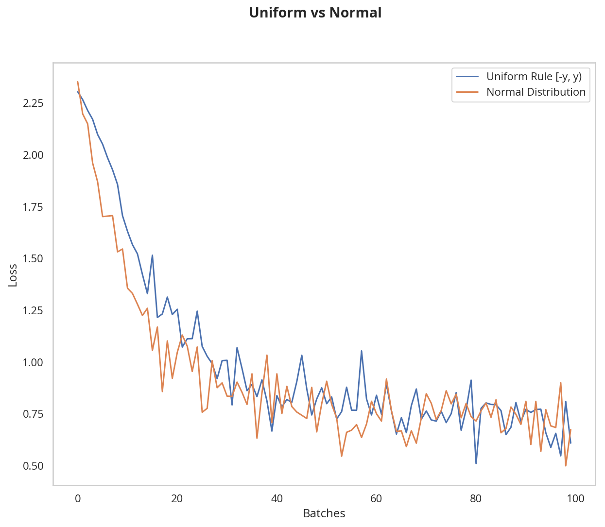
The normal distribution gives us pretty similar behavior compared to the uniform distribution, in this case. This is likely because our network is so small; a larger neural network will pick more weight values from each of these distributions, magnifying the effect of both initialization styles. In general, a normal distribution will result in better performance for a model.
Automatic Initialization
Let's quickly take a look at what happens without any explicit weight initialization.
Instantiate a model with no explicit weight initialization
evaluate the behavior using helpers
model_normal_rule = Net()
model_normal_rule.apply(weights_init_normal)
model_default = Net()
model_rule = Net()
model_rule.apply(weights_init_uniform_rule)

plot_models("Default vs Normal vs General Rule", (
    (model_default, "Default"),
    (model_normal_rule, "Normal"),
    (model_rule, "General Rule")))
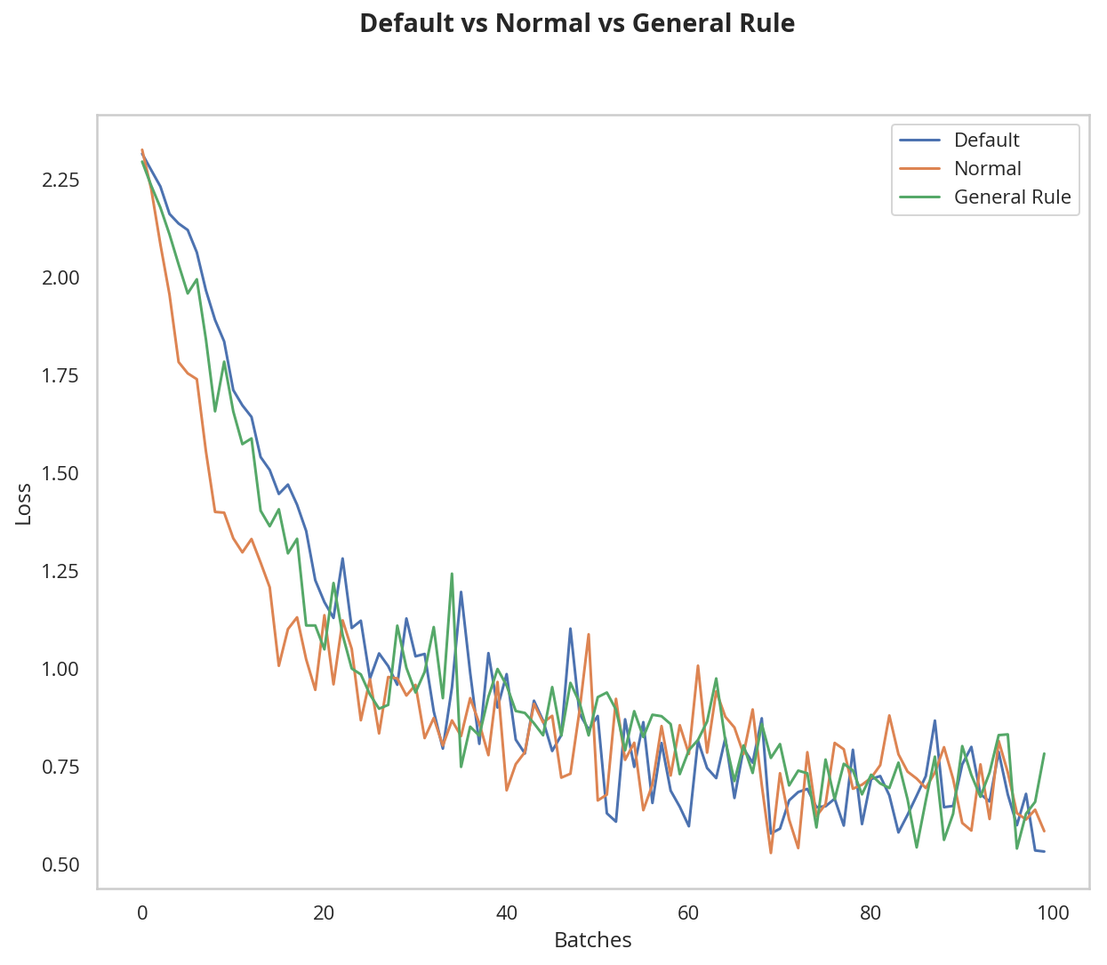
They all sort of look the same at this point.