Gradient Descent Practice
Table of Contents
This will implement the basic functions of the Gradient Descent algorithm to find the boundary in a small dataset.
Imports
From Pypi
import matplotlib.pyplot as pyplot
import numpy
import pandas
import seaborn
This Project
from neurotic.tangles.data_paths import DataPath
Helpers
For Plotting
Plot Points
This first function is used to plot the data points as a scatter plot.
def plot_points(X, y, axe=None):
    """Makes a scatter plot

    Args:
     X: array of inputs
     y: array of labels (1's and 0's)
     axe: matplotlib axis object

    Return:
     axe: matplotlib axis
    """
    admitted = X[numpy.argwhere(y==1)]
    rejected = X[numpy.argwhere(y==0)]
    if axe is None:
        figure, axe = pyplot.subplots(figsize=FIGURE_SIZE)
    axe.set_xlim((0, 1))
    axe.set_ylim((0, 1))
    axe.scatter([s[0][0] for s in rejected],
                [s[0][1] for s in rejected],
                s=25, color="blue", edgecolor="k",
                label="Rejects")
    axe.scatter([s[0][0] for s in admitted],
                   [s[0][1] for s in admitted],
                   s=25, color='red', edgecolor='k', label="Accepted")
    axe.legend()
    return axe
Display
The somewhat obscurely named display function is used to plot the separation lines of our model.
def display(m, b, color='g--', axe=None):
    """Makes a line plot

    Args:
     m: slope for the line
     b: intercept for the line
     color: color and line type for plot
     axe: matplotlib axis

    Return:
     axe: matplotlib axis
    """
    if axe is None:
        figure, axe = pyplot.subplots(figsize=FIGURE_SIZE)
    x = numpy.arange(-10, 10, 0.1)
    axe.plot(x, m*x+b, color)
    return axe
%matplotlib inline
seaborn.set(style="whitegrid")
FIGURE_SIZE = (14, 12)
The Data
We'll load the data from data.csv which has three columns - the first two are the inputs and the third is the label that we are trying to predict for the inputs.
path = DataPath("data.csv")
My setup is a little different than the Udacity setup so I'm going to have to get into the habit of setting the file before submission.
print(path.from_folder)
DATA_FILE = path.from_folder
../../../data/introduction_to_neural_networks/data.csv
I'm not sure exactly why, but the data is loaded as a pandas DataFrame (with read_csv) and then converted into two arrays.
data = pandas.read_csv(DATA_FILE, header=None)
X_train = numpy.array(data[[0,1]])
y_train = numpy.array(data[2])
| Data | Rows | Columns |
|---|---|---|
| X | 100 | 2 |
| y | 100 | N/A |
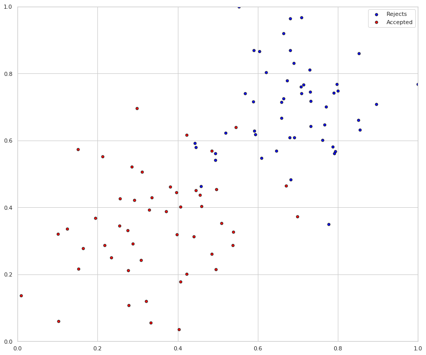
Here's what our data looks like. I don't know what the inputs represent so I didn't label the axes, but it is a plot of the first input variable vs the second input variable, with the colors determined by the labels (y-values).
axe = plot_points(X_train,y_train)
The Basic Functions
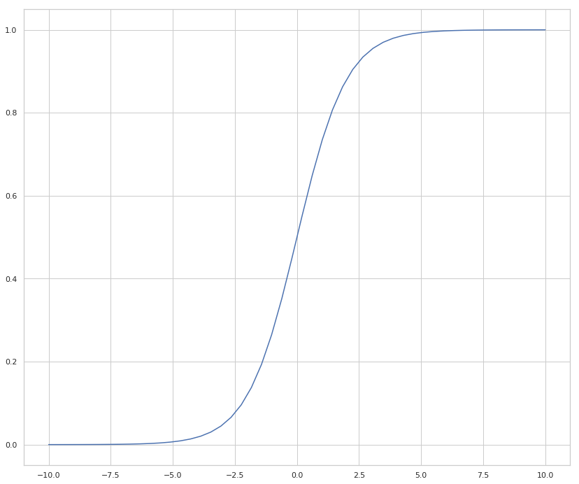
The Sigmoid activation function
This is the function that pushes the probabilities that are produced to be close to 1 or 0 so we can classify the inputs.
\[\sigma(x) = \frac{1}{1+e^{-x}}\]
def sigmoid(x: numpy.ndarray) -> numpy.ndarray:
    """Calculates the sigmoid of x

    Args:
     x: input to classify

    Returns:
     sigmoid of x
    """
    return 1/(1 + numpy.exp(-x))
figure, axe = pyplot.subplots(figsize=FIGURE_SIZE)
x = numpy.linspace(-10, 10)
y = sigmoid(x)
lines = axe.plot(x, y)
Output (prediction) formula
This function takes the dot product of the weights and inputs and adds the bias before returning the sigmoid of the calculation.
\[\hat{y} = \sigma(w_1 x_1 + w_2 x_2 + b)\]
def output_formula(features: numpy.ndarray,
                   weights: numpy.ndarray,
                   bias: numpy.ndarray) -> numpy.ndarray:
    """Predicts the outcomes for the inputs

    Args:
     features: inputs variables
     weights: array of weights for the variables
     bias: array of constants to adjust the output

    Returns:
     an array of predicted labels for the inputs
    """
    return sigmoid(features.dot(weights.T) + bias)
Error function (log-loss)
This is used for reporting, since the actual updating of the weights uses the gradient.
\[Error(y, \hat{y}) = - y \log(\hat{y}) - (1-y) \log(1-\hat{y})\]
def error_formula(y: numpy.ndarray, output: numpy.ndarray) -> numpy.ndarray:
    """Calculates the amount of error

    Args:
     y: the true labels
     output: the predicted labels

    Returns:
     amount of error in the output
    """
    return -y * numpy.log(output) - (1 - y) * numpy.log(1 - output)
The function that updates the weights (the gradient descent step)
This makes a prediction of the labels based on the inputs (using output_formula) and then updates the weights and bias based on the amount of error it had in the predictions.
\[ w_i \longrightarrow w_i + \alpha (y - \hat{y}) x_i\\ b \longrightarrow b + \alpha (y - \hat{y})\\ \]
Where \(\alpha\) is our learning rate and \(\hat{y}\) is our prediction for y.
def update_weights(x, y, weights, bias, learning_rate) -> tuple:
    """Updates the weights based on the amount of error

    Args:
     x: inputs
     y: actual labels
     weights: amount to weight each input
     bias: constant to adjust the output
     learning_rate: how much to adjust the weights

    Return:
     w, b: the updated weights
    """
    y_hat = output_formula(x, weights, bias)
    weights +=  learning_rate * (y - y_hat) * x
    bias += learning_rate * (y - y_hat)
    return weights, bias
Training function
This function will help us iterate the gradient descent algorithm through all the data, for a number of epochs. It will also plot the data, and some of the boundary lines obtained as we run the algorithm.
numpy.random.seed(44)
epochs = 100
learning_rate = 0.01
def train(features, targets, epochs, learning_rate, graph_lines=False) -> tuple:
    """Trains a model using gradient descent

    Args:
     features: matrix of inputs
     targets: array of labels for the inputs
     epochs: number of times to train the model
     learning_rate: how much to adjust the weights per epoch

    Returns:
     weights, bias, errors, plot_x, plot_y: What we learned and how we improved
    """
    errors = []
    n_records, n_features = features.shape
    last_loss = None
    weights = numpy.random.normal(scale=1 / n_features**.5, size=n_features)
    bias = 0
    plot_x, plot_y = [], []
    for epoch in range(epochs):
        # train on each row in the training data
        for x, y in zip(features, targets):
            output = output_formula(x, weights, bias)
            error = error_formula(y, output)
            weights, bias = update_weights(x, y, weights, bias, learning_rate)

        # Printing out the log-loss error on the training set
        out = output_formula(features, weights, bias)
        loss = numpy.mean(error_formula(targets, out))
        errors.append(loss)
        if epoch % (epochs / 10) == 0:
            print("\n========== Epoch {} ==========".format(epoch))
            if last_loss and last_loss < loss:
                print("Training loss: ", loss, "  WARNING - Loss Increasing")
            else:
                print("Training loss: ", loss)
            last_loss = loss
            predictions = out > 0.5
            accuracy = numpy.mean(predictions == targets)
            print("Accuracy: ", accuracy)
        if graph_lines and epoch % (epochs / 100) == 0:
            plot_x.append(-weights[0]/weights[1])
            plot_y.append(-bias/weights[1])
    return weights, bias, errors, plot_x, plot_y
Time to train the algorithm.
When we run the function, we'll obtain the following:
- 10 updates with the current training loss and accuracy
- A plot of the data and some of the boundary lines obtained. The final one is in black. Notice how the lines get closer and closer to the best fit, as we go through more epochs.
- A plot of the error function. Notice how it decreases as we go through more epochs.
weights, bias, errors, plot_x, plot_y = train(X_train, y_train, epochs, learning_rate, True)
========== Epoch 0 ==========
Training loss:  0.7135845195381634
Accuracy:  0.4

========== Epoch 10 ==========
Training loss:  0.6225835210454962
Accuracy:  0.59

========== Epoch 20 ==========
Training loss:  0.5548744083669508
Accuracy:  0.74

========== Epoch 30 ==========
Training loss:  0.501606141872473
Accuracy:  0.84

========== Epoch 40 ==========
Training loss:  0.4593334641861401
Accuracy:  0.86

========== Epoch 50 ==========
Training loss:  0.42525543433469976
Accuracy:  0.93

========== Epoch 60 ==========
Training loss:  0.3973461571671399
Accuracy:  0.93

========== Epoch 70 ==========
Training loss:  0.3741469765239074
Accuracy:  0.93

========== Epoch 80 ==========
Training loss:  0.35459973368161973
Accuracy:  0.94

========== Epoch 90 ==========
Training loss:  0.3379273658879921
Accuracy:  0.94
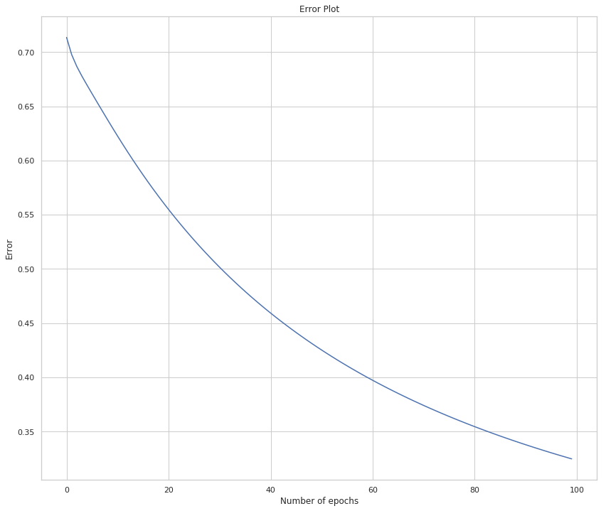
As you can see from the output the accuracy is getting better while the training loss (the mean of the error) is going down.
# Plotting the solution boundary
figure, axe = pyplot.subplots(figsize=FIGURE_SIZE)
axe.set_title("Solution boundary")
learning = zip(plot_x, plot_y)
for learn_x, learn_y in learning:
    display(learn_x, learn_y, axe=axe)
axe = display(-weights[0]/weights[1], -bias/weights[1], 'black', axe)

# Plotting the data
axe = plot_points(X_train, y_train, axe)
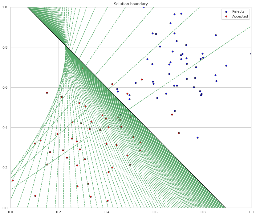
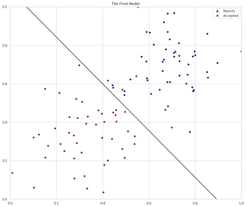
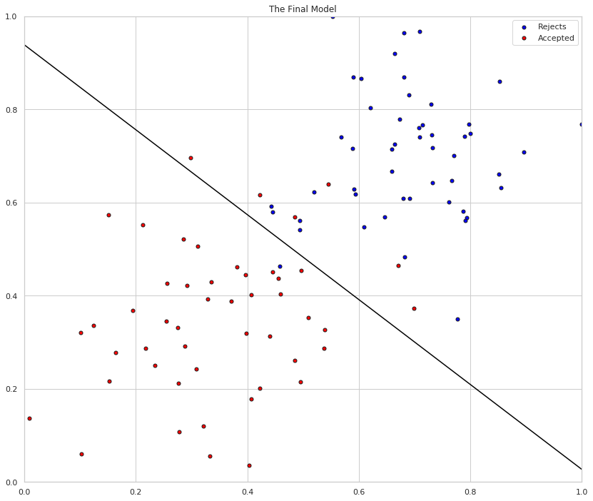
The green lines are the boundary as the model is trained, the black line is the final separator. While pretty, the green lines kind of obscure how well the sepration did. Here's just the final line with the input data.
# Plotting the solution boundary
figure, axe = pyplot.subplots(figsize=FIGURE_SIZE)
axe.set_title("The Final Model")
axe = display(-weights[0]/weights[1], -bias/weights[1], 'black', axe)

# Plotting the data
axe = plot_points(X_train, y_train, axe)
Finally, this is the amount of error as the model is trained.
# Plotting the error
figure, axe = pyplot.subplots(figsize=FIGURE_SIZE)
axe.set_title("Error Plot")
axe.set_xlabel('Number of epochs')
axe.set_ylabel('Error')
axe = axe.plot(errors)
Simpler Training
If you squint at the train function you might notice that a considerable amount of it is used for reporting, making it a little harder to read than necessary. This is the same function without the extra reporting.
def only_train(features, targets, epochs, learning_rate) -> tuple:
    """Trains a model using gradient descent

    Args:
     features: matrix of inputs
     targets: array of labels for the inputs
     epochs: number of times to train the model
     learning_rate: how much to adjust the weights per epoch

    Returns:
     weights, bias: Our final model
    """
    number_of_records, number_of_features = features.shape
    weights = numpy.random.normal(scale=1/number_of_records**.5,
                                  size=number_of_features)
    bias = 0
    for epoch in range(epochs):
        for x, y in zip(features, targets):
            weights, bias = update_weights(x, y, weights, bias, learning_rate)
    return weights, bias
weights, bias = only_train(X_train, y_train, epochs, learning_rate)
# Plotting the solution boundary
figure, axe = pyplot.subplots(figsize=FIGURE_SIZE)
axe.set_title("The Final Model")
axe = display(-weights[0]/weights[1], -bias/weights[1], 'black', axe)

# Plotting the data
axe = plot_points(X_train, y_train, axe)
And the model for our linear classifier:
print(("\\[\nw_0 x_0 + w_1 x_1 + b "
       "= {:.2f}x_0 + {:.2f}x_1 + {:.2f}\n\\]").format(weights[0],
                                                       weights[1],
                                                       bias))
\[ w_0 x_0 + w_1 x_1 + b = -3.13x_0 + -3.62x_1 + 3.31 \]