Student Admissions
Table of Contents
- Introduction
- Imports
- Some Set Up
- Loading the data
- Plotting the data
- One-Hot Encoding the Rank
- Scaling the data
- Splitting the data into Training and Testing
- Splitting the data into features and targets (labels)
- Training the 2-layer Neural Network
- Backpropagate the error
- Calculating the Accuracy on the Test Data
Introduction
In this notebook, I'll student admissions to graduate school at UCLA based on three pieces of data:
- GRE Scores (Test)
- GPA Scores (Grades)
- Class rank (1-4)
The dataset originally came from here: http://www.ats.ucla.edu/ (although I couldn't find it).
Imports
From python
from functools import partial
From PyPi
from tabulate import tabulate
import matplotlib.pyplot as pyplot
import numpy
import pandas
import seaborn
This Project
from neurotic.tangles.data_paths import DataPath
Some Set Up
Tables
table = partial(tabulate, showindex=False, tablefmt='orgtbl', headers="keys")
Plotting
%matplotlib inline
seaborn.set(style="whitegrid")
FIGURE_SIZE = (14, 12)
Loading the data
path = DataPath("student_data.csv")
print(path.from_folder)
../../../data/introduction-to-neural-networks/student_data.csv
data = pandas.read_csv(path.from_folder)
print(table(data.head()))
| admit | gre | gpa | rank |
|---|---|---|---|
| 0 | 380 | 3.61 | 3 |
| 1 | 660 | 3.67 | 3 |
| 1 | 800 | 4 | 1 |
| 1 | 640 | 3.19 | 4 |
| 0 | 520 | 2.93 | 4 |
print(table(data.describe(), showindex=True))
| admit | gre | gpa | rank | |
|---|---|---|---|---|
| count | 400 | 400 | 400 | 400 |
| mean | 0.3175 | 587.7 | 3.3899 | 2.485 |
| std | 0.466087 | 115.517 | 0.380567 | 0.94446 |
| min | 0 | 220 | 2.26 | 1 |
| 25% | 0 | 520 | 3.13 | 2 |
| 50% | 0 | 580 | 3.395 | 2 |
| 75% | 1 | 660 | 3.67 | 3 |
| max | 1 | 800 | 4 | 4 |
So we have 400 applicants with about 32% of them being admitted. I don't know how to interpret the rank, maybe that's the quarter the student was in.
Plotting the data
First let's make a plot of our data to see how it looks. In order to have a 2D plot, let's ingore the rank.
Plot Points
def plot_points(data: pandas.DataFrame, identifier: str="All"):
    """Plots the GRE vs GPA

    Args:
     data: frame with the admission, GRE, and GPA data
     identifier: something to identify the data set
    """
    figure, axe = pyplot.subplots(figsize=FIGURE_SIZE)
    axe.set_title("GRE vs GPA and Admissions to UCLA Graduate School ({})".format(identifier))
    X = numpy.array(data[["gre","gpa"]])
    y = numpy.array(data["admit"])
    admitted = X[numpy.argwhere(y==1)]
    rejected = X[numpy.argwhere(y==0)]
    axe.scatter([s[0][0] for s in rejected], [s[0][1] for s in rejected],
                s = 25, color = 'red', edgecolor = 'k', label="Rejected")
    axe.scatter([s[0][0] for s in admitted], [s[0][1] for s in admitted],
                s = 25, color = 'cyan', edgecolor = 'k', label="Admitted")
    axe.set_xlabel('Test (GRE)')
    axe.set_ylabel('Grades (GPA)')
    axe.legend()
    return
GRE Vs GPA
plot_points(data)
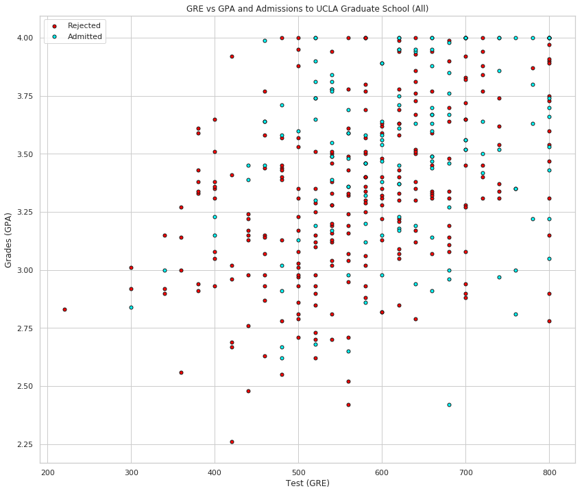
Roughly, it looks like the students with high scores in the grades and test passed, while the ones with low scores didn't, but the data is not as nicely separable as we hoped it would be (to say the least). Maybe it would help to take the rank into account? Let's make 4 plots, each one for each rank.
By Rank
Separating the ranks
data_rank_1 = data[data["rank"]==1]
data_rank_2 = data[data["rank"]==2]
data_rank_3 = data[data["rank"]==3]
data_rank_4 = data[data["rank"]==4]
plot_points(data_rank_1, "Rank 1")
![]()
plot_points(data_rank_2, "Rank 2")
![]()
plot_points(data_rank_3, "Rank 3")
![]()
plot_points(data_rank_4, "Rank 4")
![]()
ranked = data.groupby("rank").sum()
fraction = (ranked/data.admit.sum()).reset_index()
print(table(fraction[["rank", "admit"]]))
| rank | admit |
|---|---|
| 1 | 0.259843 |
| 2 | 0.425197 |
| 3 | 0.220472 |
| 4 | 0.0944882 |
figure, axe = pyplot.subplots(figsize=FIGURE_SIZE)
axe.set_title("Fraction Admitted By Rank")
axe = fraction.plot.bar(x="rank", y="admit", ax=axe, rot=False)
![]()
This looks more promising, as it seems that the lower the rank, the higher the acceptance rate (with rank 2 being the dominant rank among the admitted). Let's use the rank as one of our inputs. In order to do this, we should one-hot encode it.
One-Hot Encoding the Rank
We'll do the one-hot-encoding using pandas' get_dummies function.
one_hot_data = pandas.get_dummies(data, columns=["rank"])
print(table(one_hot_data.head()))
| admit | gre | gpa | rank_1 | rank_2 | rank_3 | rank_4 |
|---|---|---|---|---|---|---|
| 0 | 380 | 3.61 | 0 | 0 | 1 | 0 |
| 1 | 660 | 3.67 | 0 | 0 | 1 | 0 |
| 1 | 800 | 4 | 1 | 0 | 0 | 0 |
| 1 | 640 | 3.19 | 0 | 0 | 0 | 1 |
| 0 | 520 | 2.93 | 0 | 0 | 0 | 1 |
Scaling the data
The next step is to scale the data. We notice that the range for grades is 1.0-4.0, whereas the range for test scores is roughly 200-800, which is much larger. This means our data is skewed, and that makes it hard for a neural network to handle. Let's fit our two features into a range of 0-1, by dividing the grades by 4.0, and the test score by 800.
Making a copy of our data
processed_data = one_hot_data[:]
Scale the columns
processed_data["gpa"] = one_hot_data["gpa"]/4
processed_data["gre"] = one_hot_data["gre"]/800
print(table(processed_data.head()))
| admit | gre | gpa | rank_1 | rank_2 | rank_3 | rank_4 |
|---|---|---|---|---|---|---|
| 0 | 0.475 | 0.9025 | 0 | 0 | 1 | 0 |
| 1 | 0.825 | 0.9175 | 0 | 0 | 1 | 0 |
| 1 | 1 | 1 | 1 | 0 | 0 | 0 |
| 1 | 0.8 | 0.7975 | 0 | 0 | 0 | 1 |
| 0 | 0.65 | 0.7325 | 0 | 0 | 0 | 1 |
Splitting the data into Training and Testing
In order to test our algorithm, we'll split the data into a Training and a Testing set by sampling the data's index (using numpy.random.choice) to find the training set and dropping the sample (pandas.DataFrame.drop) from the data to create the test set. The size of the testing set will be 10% of the total data.
training_size = int(len(processed_data) * 0.9)
sample = numpy.random.choice(processed_data.index,
                             size=training_size, replace=False)
train_data, test_data = processed_data.iloc[sample], processed_data.drop(sample)
print("Number of training samples is", len(train_data))
print("Number of testing samples is", len(test_data))
Number of training samples is 360
Number of testing samples is 40
print(table(train_data[:10]))
| admit | gre | gpa | rank_1 | rank_2 | rank_3 | rank_4 |
|---|---|---|---|---|---|---|
| 0 | 0.85 | 0.77 | 0 | 0 | 0 | 1 |
| 1 | 0.7 | 0.745 | 1 | 0 | 0 | 0 |
| 0 | 0.775 | 0.7625 | 0 | 1 | 0 | 0 |
| 0 | 0.825 | 0.8975 | 0 | 0 | 1 | 0 |
| 0 | 0.75 | 0.85 | 0 | 0 | 1 | 0 |
| 1 | 0.65 | 0.975 | 0 | 0 | 1 | 0 |
| 0 | 0.775 | 0.8325 | 0 | 0 | 1 | 0 |
| 0 | 0.875 | 0.8175 | 0 | 1 | 0 | 0 |
| 0 | 0.475 | 0.835 | 0 | 0 | 1 | 0 |
| 0 | 0.725 | 0.84 | 0 | 1 | 0 | 0 |
print(table(test_data[:10]))
| admit | gre | gpa | rank_1 | rank_2 | rank_3 | rank_4 |
|---|---|---|---|---|---|---|
| 0 | 0.5 | 0.77 | 0 | 1 | 0 | 0 |
| 0 | 0.875 | 0.77 | 0 | 1 | 0 | 0 |
| 1 | 0.875 | 1 | 1 | 0 | 0 | 0 |
| 0 | 0.65 | 0.8225 | 1 | 0 | 0 | 0 |
| 0 | 0.45 | 0.785 | 1 | 0 | 0 | 0 |
| 1 | 0.75 | 0.7875 | 0 | 1 | 0 | 0 |
| 1 | 0.725 | 0.865 | 0 | 1 | 0 | 0 |
| 1 | 0.775 | 0.795 | 0 | 1 | 0 | 0 |
| 0 | 0.725 | 1 | 0 | 1 | 0 | 0 |
| 1 | 0.55 | 0.8625 | 0 | 1 | 0 | 0 |
Splitting the data into features and targets (labels)
Now, as a final step before the training, we'll split the data into features (X) and targets (y).
features = train_data.drop('admit', axis="columns")
targets = train_data['admit']
features_test = test_data.drop('admit', axis="columns")
targets_test = test_data['admit']
print(table(features[:10]))
| gre | gpa | rank_1 | rank_2 | rank_3 | rank_4 |
|---|---|---|---|---|---|
| 0.85 | 0.77 | 0 | 0 | 0 | 1 |
| 0.7 | 0.745 | 1 | 0 | 0 | 0 |
| 0.775 | 0.7625 | 0 | 1 | 0 | 0 |
| 0.825 | 0.8975 | 0 | 0 | 1 | 0 |
| 0.75 | 0.85 | 0 | 0 | 1 | 0 |
| 0.65 | 0.975 | 0 | 0 | 1 | 0 |
| 0.775 | 0.8325 | 0 | 0 | 1 | 0 |
| 0.875 | 0.8175 | 0 | 1 | 0 | 0 |
| 0.475 | 0.835 | 0 | 0 | 1 | 0 |
| 0.725 | 0.84 | 0 | 1 | 0 | 0 |
print(table(dict(admit=targets[:10])))
| admit |
|---|
| 0 |
| 1 |
| 0 |
| 0 |
| 0 |
| 1 |
| 0 |
| 0 |
| 0 |
| 0 |
Training the 2-layer Neural Network
The following function trains the 2-layer neural network. First, we'll write some helper functions.
Helper Functions
def sigmoid(x):
    return 1 / (1 + numpy.exp(-x))
and the derivative of the sigmoid.
def sigmoid_prime(x):
    return sigmoid(x) * (1-sigmoid(x))
def error_formula(y, output):
    return - y * numpy.log(output) - (1 - y) * numpy.log(1-output)
Backpropagate the error
Now it's your turn to shine. Write the error term. Remember that this is given by the equation \[ -(y-\hat{y}) \sigma'(x) \]
def error_term_formula(y, output):
    return (y - output) * output * (1 - output)
Training
epochs = 1000
learn_rate = 0.5
Training function
def train_nn(features, targets, epochs, learnrate):

    # Use to same seed to make debugging easier
    numpy.random.seed(42)

    n_records, n_features = features.shape
    last_loss = None

    # Initialize weights
    weights = numpy.random.normal(scale=1 / n_features**.5, size=n_features)

    for e in range(epochs):
        del_w = numpy.zeros(weights.shape)
        for x, y in zip(features.values, targets):
            # Loop through all records, x is the input, y is the target

            # Activation of the output unit
            #   Notice we multiply the inputs and the weights here
            #   rather than storing h as a separate variable
            output = sigmoid(numpy.dot(x, weights))

            # The error, the target minus the network output
            error = error_formula(y, output)

            # The error term
            #   Notice we calulate f'(h) here instead of defining a separate
            #   sigmoid_prime function. This just makes it faster because we
            #   can re-use the result of the sigmoid function stored in
            #   the output variable
            error_term = error_term_formula(y, output)

            # The gradient descent step, the error times the gradient times the inputs
            del_w += error_term * x

        # Update the weights here. The learning rate times the
        # change in weights, divided by the number of records to average
        weights += learnrate * del_w / n_records

        # Printing out the mean square error on the training set
        if e % (epochs / 10) == 0:
            out = sigmoid(numpy.dot(features, weights))
            loss = numpy.mean((out - targets) ** 2)
            print("Epoch:", e)
            if last_loss and last_loss < loss:
                print("Train loss: ", loss, "  WARNING - Loss Increasing")
            else:
                print("Train loss: ", loss)
            last_loss = loss
            print("=========")
    print("Finished training!")
    return weights
weights = train_nn(features, targets, epochs, learn_rate)
Epoch: 0
Train loss:  0.27247853979302755
=========
Epoch: 100
Train loss:  0.20397593223991445
=========
Epoch: 200
Train loss:  0.2014297690420066
=========
Epoch: 300
Train loss:  0.2003513187214578
=========
Epoch: 400
Train loss:  0.19984320017443669
=========
Epoch: 500
Train loss:  0.19956325048732546
=========
Epoch: 600
Train loss:  0.19938027609704898
=========
Epoch: 700
Train loss:  0.1992416788675009
=========
Epoch: 800
Train loss:  0.19912513146497982
=========
Epoch: 900
Train loss:  0.19902058341953008
=========
Finished training!
Calculating the Accuracy on the Test Data
test_out = sigmoid(numpy.dot(features_test, weights))
predictions = test_out > 0.5
accuracy = numpy.mean(predictions == targets_test)
print("Prediction accuracy: {:.3f}".format(accuracy))
Prediction accuracy: 0.575
Not horrible, considering the test-set, but not great either.
Try More Epochs
weights_2 = train_nn(features, targets, epochs*2, learn_rate)
Epoch: 0
Train loss:  0.27247853979302755
=========
Epoch: 200
Train loss:  0.2014297690420066
=========
Epoch: 400
Train loss:  0.19984320017443669
=========
Epoch: 600
Train loss:  0.19938027609704898
=========
Epoch: 800
Train loss:  0.19912513146497982
=========
Epoch: 1000
Train loss:  0.19892324129363695
=========
Epoch: 1200
Train loss:  0.19874162735565162
=========
Epoch: 1400
Train loss:  0.19857138905455757
=========
Epoch: 1600
Train loss:  0.1984095079666442
=========
Epoch: 1800
Train loss:  0.1982546851201456
=========
Finished training!
test_out = sigmoid(numpy.dot(features_test, weights_2))
predictions = test_out > 0.5
accuracy = numpy.mean(predictions == targets_test)

print("Prediction accuracy: {:.3f}".format(accuracy))
Prediction accuracy: 0.575
It doesn't make a noticeable difference. Maybe this is the best it can do with only these features.