Training with Gradient Descent
Table of Contents
This is an example of implementing gradient descent to update the weights in a neural network.
Set Up
Imports
From PyPi
from sklearn.model_selection import train_test_split
from sklearn.preprocessing import scale
import matplotlib.pyplot as pyplot
import numpy
import pandas
import seaborn
This Project
from neurotic.tangles.data_paths import DataPath
from neurotic.tangles.helpers import org_table
Plotting
%matplotlib inline
seaborn.set(style="whitegrid",
            rc={"axes.grid": False,
                "font.family": ["sans-serif"],
                "font.sans-serif": ["Latin Modern Sans", "Lato"],
                "figure.figsize": (20, 40)},
            font_scale=2)
FIGURE_SIZE = (12, 10)
The Data
We will use data originally take from the UCLA Institute for Digital Research and Education (I couldn't find the dataset when I went to look for it). It has three features:
| Feature | Description |
|---|---|
gre |
Graduate Record Exam score |
gpa |
Grade Point Average |
rank |
Rank of the undergraduate school |
The rank is a scale from 1 to 4, with 1 being the most prestigious school and 4 being the least.
It also has one output value - admit which indicates whether the student was admitted or not.
path = DataPath("student_data.csv")
data = pandas.read_csv(path.from_folder)
print(org_table(data.head()))
| admit | gre | gpa | rank |
|---|---|---|---|
| 0 | 380 | 3.61 | 3 |
| 1 | 660 | 3.67 | 3 |
| 1 | 800 | 4 | 1 |
| 1 | 640 | 3.19 | 4 |
| 0 | 520 | 2.93 | 4 |
print(data.shape)
(400, 7)
So there are 400 applications - not a huge data set.
grid = seaborn.relplot(x="gpa", y="gre", hue="admit", col="rank",
                       data=data, col_wrap=2)
pyplot.subplots_adjust(top=0.9)
title = grid.fig.suptitle("UCLA Student Admissions", weight="bold")
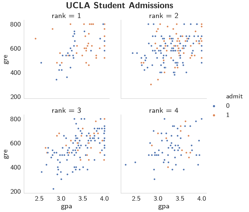
It does look like the rank of the school matters, perhaps even more than scores.
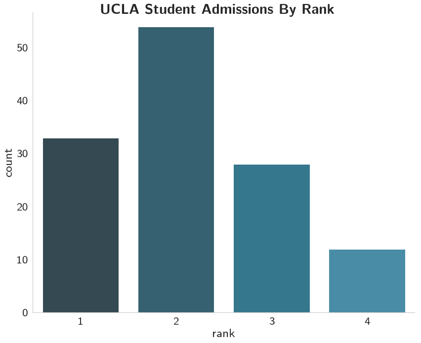
with seaborn.color_palette("PuBuGn_d"):
    grid = seaborn.catplot(x="rank", kind="count", data=data,
                           height=10, aspect=12/10)
    title = grid.fig.suptitle("UCLA Student Submissions By Rank", weight="bold")
![]()
So most of the applicants came from second and third-ranked schools.
admitted = data[data.admit==1]
with seaborn.color_palette("PuBuGn_d"):
    grid = seaborn.catplot(x="rank", kind="count", data=admitted,
                           height=10, aspect=12/10)
    title = grid.fig.suptitle("UCLA Student Admissions By Rank",
                              weight="bold")
 And it looks like most of the admitted were from first and second-ranked schools, with most coming from the second-ranked schools.
admission_rate = (admitted["rank"].value_counts(sort=False)
                  /data["rank"].value_counts(sort=False))
admission_rate = (admission_rate * 100).round(2)
admission_rate = admission_rate.reset_index()
admission_rate.columns = ["Rank", "Percent Admitted"]
print(org_table(admission_rate))
| Rank | Percent Admitted |
|---|---|
| 1 | 54.1 |
| 2 | 35.76 |
| 3 | 23.14 |
| 4 | 17.91 |
So, even though the second-tier schools had the most admitted, the top-tier school was admitted at a higher rate.
Did GRE Matter?
with seaborn.color_palette("hls"):
    grid = seaborn.catplot(x="rank", y="gre", hue="admit", data=data,
                           height=10, aspect=12/10)
    title = grid.fig.suptitle("Admissions by School Rank", weight="bold")
![]()
This one's a little tough to say, it looks like it's better to have a higher GRE, but once you get below 700 it isn't as clear, at least not to me.
What about GPA?
with seaborn.color_palette("hls"):
    grid = seaborn.catplot(x="rank", y="gpa", hue="admit", data=data,
                           height=10, aspect=12/10)
    title = grid.fig.suptitle("Admissions by School Rank", weight="bold")
![]()
This one seems even less demonstrative than GRE does.
Pre-Processing the Data
Dummy Variables
Since the rank values are ordinal, not numeric, we need to create some one-hot-encoded columns for it using get_dummies.
First I'll get some counts so I can double-check my work. Note to future self: rank is a pandas DataFrame method, so naming a column 'rank' is probably not such a great idea.
rank_counts = data["rank"].value_counts()
data = pandas.get_dummies(data, columns=["rank"], prefix="rank")
for rank in range(1, 5):
    assert rank_counts[rank] == data["rank_{}".format(rank)].sum()
print(org_table(data.head()))
| admit | gre | gpa | rank_1 | rank_2 | rank_3 | rank_4 |
|---|---|---|---|---|---|---|
| 0 | 380 | 3.61 | 0 | 0 | 1 | 0 |
| 1 | 660 | 3.67 | 0 | 0 | 1 | 0 |
| 1 | 800 | 4 | 1 | 0 | 0 | 0 |
| 1 | 640 | 3.19 | 0 | 0 | 0 | 1 |
| 0 | 520 | 2.93 | 0 | 0 | 0 | 1 |
Standardization
Now I'll convert the gre and gpa to have a mean of 0 and a variance of 1 using sklearn's scale function.
data["gre"] = scale(data.gre.astype("float64").values)
data["gpa"] = scale(data.gpa.values)
print(org_table(data.sample(5)))
| admit | gre | gpa | rank_1 | rank_2 | rank_3 | rank_4 |
|---|---|---|---|---|---|---|
| 0 | -0.240093 | -0.394379 | 0 | 0 | 0 | 1 |
| 1 | 0.973373 | 1.60514 | 1 | 0 | 0 | 0 |
| 0 | -0.413445 | -0.0260464 | 0 | 0 | 0 | 1 |
| 1 | 0.106612 | -0.631165 | 0 | 1 | 0 | 0 |
| 0 | -0.760149 | -1.52569 | 0 | 0 | 1 | 0 |
print(data.gre.mean().round())
print(data.gre.std().round())
print(data.gpa.mean().round())
print(data.gpa.std().round())
-0.0
1.0
0.0
1.0
The Error
For this we're going to use the Mean Square Error.
\[ E = \frac{1}{2m}\sum_{\mu} (y^{\mu} - \hat{y}^{\mu})^2 \]
This doesn't actually change our training, it just acts as an estimate of the error as we train so we can see that the model is getting better (hopefully).
The General Training Algorithm
- Set the weight delta to 0 (\(\Delta w_i = 0\))
- For each record in the training data:
- Make a forward pass to get the output: \(\hat{y} = f\left(\sum_{i} w_i x_i \right)\)
- Calculate the error: \(\delta = (y - \hat{y}) f'\left(\sum_i w_i x_i\right)\)
- Update the weight delta: \(\Delta w_i = \Delta w_i + \delta x_i\)
- Update the weights : \(w_i = w_i + \eta \frac{\Delta w_i}{m}\)
- Repeart for \(e\) epochs
The Numpy Implementation
I'm going to implement the previous algorithm using numpy.
Setting up the Data
We need to set up the training and testing data. The lecture uses numpy exclusively, but as with the standardization I'll cheat a little and use sklearn. The lecture uses a slightly different naming scheme from the one you normally see in the python machine learning community (e.g. X_train, y_train) which I'll stick with it so that I don't get errors just from using the wrong names. Truthfully, I kind of like these names better, although the use of the suffix _test without the use of the suffix _train seems confusing.
features_all = data.drop("admit", axis="columns")
targets_all = data.admit
The example given uses 10 % of the data for testing and 90% for training.
features, features_test, targets, targets_test = train_test_split(features_all, targets_all, test_size=0.1)
print(features.shape)
print(targets.shape)
print(features_test.shape)
print(targets_test.shape)
(360, 6)
(360,)
(40, 6)
(40,)
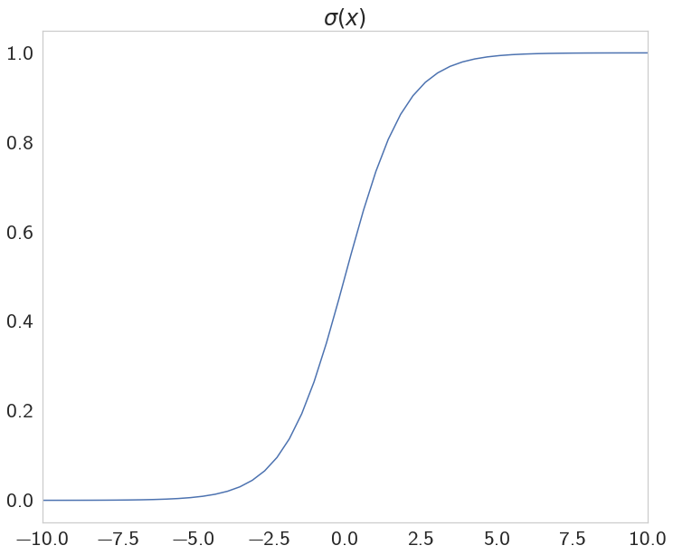
The Sigmoid
This is our activation function.
def sigmoid(x):
    """
    Calculate sigmoid
    """
    return 1 / (1 + numpy.exp(-x))
limit = [-10, 10]
x = numpy.linspace(*limit)
y = sigmoid(x)
figure, axe = pyplot.subplots(figsize=FIGURE_SIZE)
axe.set_xlim(*limit)
axe.set_title("$\sigma(x)$", weight="bold")
plot = axe.plot(x, y)
Some Setup
To make the outcome reproducible I'll set the random seed.
numpy.random.seed(17)
Now some variables need to be set up for the print output.
n_records, n_features = features.shape
last_loss = None
Initialize weights
We're going to use a normally distributed set of random weights to start with. The scale is the spread of the distribution we're sampling from. A rule-of-thumb for the spread is to use \(\frac{1}{\sqrt{n}}\) where n is the numeber of input units. This keeps the input to the sigmoid low, even as the number of inputs goes up.
weights = numpy.random.normal(scale=1/n_features**.5, size=n_features)
Set Up The Learning
Now some neural network hyperparameters - how long do we train and how fast do we learn at each pass?
epochs = 1000
learnrate = 0.5
The Training Loop
This is where we do the actual training (gradient descent).
for epoch in range(epochs):
    delta_weights = numpy.zeros(weights.shape)
    for x, y in zip(features.values, targets):
        output = sigmoid(x.dot(weights))

        error = y - output

        error_term = error * (output * (1 - output))

        delta_weights += error_term * x

    weights += (learnrate * delta_weights)/n_records

    # Printing out the mean square error on the training set
    if epoch % (epochs / 10) == 0:
        out = sigmoid(numpy.dot(features, weights))
        loss = numpy.mean((out - targets) ** 2)
        if last_loss and last_loss < loss:
            print("Train loss: ", loss, "  WARNING - Loss Increasing")
        else:
            print("Train loss: ", loss)
        last_loss = loss
Train loss:  0.31403028569037034
Train loss:  0.20839043233748233
Train loss:  0.19937544110681996
Train loss:  0.19697280538767817
Train loss:  0.19607622516320752
Train loss:  0.19567788493090374
Train loss:  0.19548034981121246
Train loss:  0.19537454797678722
Train loss:  0.19531455174429538
Train loss:  0.19527902197312702
Testing
Calculate accuracy on test data
test_out = sigmoid(numpy.dot(features_test, weights))
predictions = test_out > 0.5
accuracy = numpy.mean(predictions == targets_test)
print("Prediction accuracy: {:.3f}".format(accuracy))
Prediction accuracy: 0.750
Not great, but then again, we had a fairly small data set to start with.