Softmax

What is the Softmax Function?

With the stepwise and logistic function you are limited to binary classifications. The softmax function is a generalization of the logistic (sigmoid) function that lets you choose between multiple categories.

A classification problem

What animal did you see?

We have three animals and the probabilities that the animal you saw are the following:

  • P(duck) = 0.67
  • P(beaver) = 0.24
  • P(walrus) = 0.09

We count the occurrence of animals we see and get these counts.

Animal Count
Duck 2
Beaver 1
Walrus 0

So, how do you convert these scores into probabilities?

Standardize

One way to convert the counts to probabilities is by dividing each count by the total.

\[ P = \frac{count}{\textit{total count}} \]

The problem with this is we might not be dealing with counts and so we have to deal with negative numbers in which case the sum of the values (total count in this case) could equal zero. We need to use a function that will turn any value we have (even if it isn't a count) into a positive number.

Which function would turn every number into a positive number?

  • [ ] sin
  • [ ] cos
  • [ ] log
  • [X] exp

The Exponential

It turns out that if you take the numbers and use them as the power of e, your values will always be positive, so to normalize our values, instead of taking the count divided by the sum of the counts, we would take the exponential of our count divided by the sum of the exponentials of all the counts.

\[ P(duck) = \frac{e^2}{e^2 + e^1 + e^0}\\ = 0.67 \]

This is the softmax function.

Implementation

Imports

import numpy

Write a function that takes as input a list of numbers, and returns the list of values given by the softmax function. This uses numpy.exp to approximate e.

def softmax(L):
    """calculates the softmax probmabilities

    Args:
     L: List of values

    Returns:
     softmax: the softmax probabilities for the values
    """
    values = numpy.exp(L)
    return values/values.sum()
values = [2, 1, 0]
expected_values = [0.67, 0.24, 0.09]
actual = softmax(values)
tolerance = 0.1**2
expected_actual = zip(expected_values, actual)
for index, (expected, actual) in enumerate(expected_actual):
    print("{:.2f}".format(actual))
    assert abs(actual - expected) < tolerance,\
        "Expected: {} Actual: {}".format(expected, actual)
0.67
0.24
0.09
Non-Linear Regions

What's this about?

The perceptron seems to work fairly well with our admissions problem, but that's because our data is seperable with a straight line. What if we need a curved line? This should also work, the secret sauce is how we define our error function.

Continuous vs Discrete

It turns out that if your values are discrete (rather than continuous) you might have a very difficult time tuning the algorithm, because our learning rate will keep it vascillating between solutions, so for this to work, we need a continuous solution space.

Gradent Descent

Using descending a mountain as a metaphor, our goal is to look around and find the path that will take us the furthest down the mountain. In mathematical terms this means searching in the space adjacent to where we are and finding the solution that gives us the greatest reduction in error.

Discrete Vs Continuous Again (The Sigmoid)

Our categorizations are discrete, but our model doesn't work for discrete values… how do we reconcile this? The trick is to use continuous values and then, instead of using the stepwise function to classify the outcomes, we use the sigmoid function. This converts interpretation from a discrete 0 or 1 to a probability.

\[ \sigma(x) = \frac{1}{1 + e^{-x}} \]

Question

The score is defined as \(4x_1 + 5x_2 - 9\), which of the following values has a 50% probability of being blue or red?

Imports

python standard library

from math import exp
def probability(x):
    return 4 * x[0] + 5 * x[1] - 9
def sigmoid(x):
    return 1/(1+exp(-x))
inputs = [[1,1], [2, 4], [5, -5], [-4, 5]]
for x in inputs:
    p = probability(x)
    print("{}: {}".format(x, sigmoid(p)))
[1, 1]: 0.5
[2, 4]: 0.9999999943972036
[5, -5]: 8.315280276641321e-07
[-4, 5]: 0.5

The Perceptron Algorithm

The Algorithm

  1. Start with random weights. \(Wb\)
  2. Test the weights and for every misclassified point:
    • create a vector with the coordinates of the point and append a 1 to it
    • multiply the vector by the learning rate
    • If the prediction was 0, add the vector to the weights
    • If the prediction was 1, subtract the vector from the weights
  3. Stop when the stopping condition has been reached:
    • no misclassified points
    • few enough misclassified points
    • you've run long enough

Imports

From PyPi

import matplotlib.pyplot as pyplot
import numpy
import pandas
import seaborn

This Project

from neurotic.tangles.data_paths import DataPath

Setup

The Plotting

%matplotlib inline
seaborn.set(style="whitegrid")
FIGURE_SIZE = (14, 12)

The Data

path = DataPath("admissions.csv")
data = pandas.read_csv(path.from_folder)
print(data.describe())

I added the labels to match the earlier admissions problem, there aren't any in the actual data set.

Here is a plot of what we need to train our Perceptron on to create a linear classifier.

figure, axe = pyplot.subplots(figsize=FIGURE_SIZE)
accepted = data[data.Label==1]
rejected = data[data.Label==0]
axe.set_title("Admissions Data")
axe.set_xlabel("Grades")
axe.set_ylabel("Test")
axe.scatter(accepted.Grades, accepted.Test, label="Accepted")
axe.scatter(rejected.Grades, rejected.Test, label="Rejected")
legend = axe.legend()

The Implementation

Set the random seed so the outcome is reproducible

numpy.random.seed(42)

The Step Function

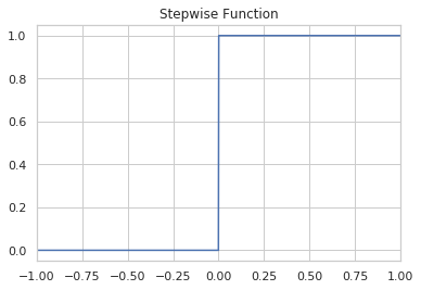
This is the stepwise function that decides if the output is a 1 or a 0.

\[ \hat{y} = \begin{cases} 1 \text{ if } Wx + b \geq 0\\ 0 \text{ if } Wx + b \lt 0 \end{cases} \]

def stepwise(value):
    """A function to convert the value to a label

    Args:
     value: number to evaluate

    Returns:
     label: 0 or 1 based on the value
    """
    return 1 if value >= 0 else 0
figure, axe = pyplot.subplots()
axe.set_title("Stepwise Function")
axe.set_xlim((-1, 1))
x = numpy.linspace(-1, 1, 1000)
y = [stepwise(value) for value in x]
line = axe.plot(x, y)

stepwise.png

The Prediction

\[ Wx + b = 0\\ \]

def prediction(X, W, b):
    """Predicts whether X is 0 or 1

    Args:
     X: matrix of inputs
     W: weights
     b: bias

    Returns:
     label: 0 or 1
    """
    return stepwise((numpy.matmul(X, W) + b)[0])

The Perceptron Step

This is where the Perceptron Trick as described in the algorithm above is implemented.

def perceptron_step(X, y, W, b, learn_rate = 0.01):
    """Adjusts the weights using the Perceptron Trick

    Args:
     X: the input data - array of rows with two columns
     y: the labels - array with one row of length matching the rows in X
     W: the weights - array of shape (2, 1)
     b: the bias - scalar
     learn_rate: how much to adjust the weights at each step

    Returns:
     W,b: the new weights and bias
    """
    for row in range(X.shape[0]):
        predicted = prediction(X[row], W, b)
        actual = y[row]
        direction = actual - predicted
        W = W + direction * learn_rate * W
        b = b + direction * learn_rate
    return W, b

The Perceptron

class Perceptron:
    """A perceptron to classify points

    Args:
     x_train: training data
     y_train: labels for the tranining data
     learnining_rate: how fast to update during training
     epochs: how many times to run the training
     verbosity: level of output
    """
    def __init__(self, x_train: numpy.ndarray, y_train: numpy.ndarray,
                 learning_rate: float=0.1, epochs: int=25,
                 verbosity: int=0):
        self.x_train = x_train
        self.y_train = y_train
        self.learning_rate = learning_rate
        self.epochs = epochs
        self.verbosity = verbosity
        self._weights = None
        self._bias = None
        self._training_data = None
        return

    @property
    def training_data(self) -> pandas.DataFrame:
        """the training data as a DataFrame"""
        if self._training_data is None:
            self._training_data = pandas.DataFrame(self.x_train)
        return self._training_data

    @property
    def weights(self) -> numpy.ndarray:
        """Vector of weights for the predictions"""
        if self._weights is None:
            self._weights = numpy.array(numpy.random.rand(self.x_train[0].shape[0], 1))
        return self._weights

    @weights.setter
    def weights(self, weights_prime: numpy.ndarray) -> None:
        """Update the weight

       Args:
        weights: new weights for the prediction calculations
       """
        self._weights = weights_prime
        return

    @property
    def bias(self) -> float:
        """The bias constant"""
        if self._bias is None:
            self._bias = numpy.random.rand(1)[0] + max(self.x_train.T[0])
        return self._bias

    @bias.setter
    def bias(self, bias_prime: float) -> None:
        """Sets the bias for predictions"""
        self._bias = bias_prime
        return

    def separator(self, x: float) -> float:
        """For the two-dimensional case, gives the y-value 

       Returns:
        the y-value for the separator line
       """
        return -(self.weights[0] * x + self.bias)/self.weights[1]

    def predict(self, instance: numpy.ndarray) -> int:
        """makes a prediction for a single point

       Args:
        instance: data to make a prediction for

       Returns:
        prediction: a 0 or 1
       """
        score = (numpy.matmul(instance, self.weights) + self.bias)[0]
        return 1 if score >= 0 else 0

    def take_step(self):
        """takes a single training step"""
        for row in range(self.x_train.shape[0]):
            predicted = self.predict(self.x_train[row])
            actual = self.y_train[row]
            direction = actual - predicted
            self.weights = (self.weights.T
                            + direction * self.learning_rate * self.x_train[row]).T
            self.bias = self.bias + direction * self.learning_rate
            if self.verbosity > 1:
                print("Predicted: {}".format(predicted))
                print("Actual: {}".format(actual))
                print("Direction: {}".format(direction))
                print("Weights: {}".format(self.weights))
                print("Bias: {}".format(self.bias))
        return

    def train(self):
        """Trains the perceptron"""
        if self.verbosity > 0:
            print("Starting Training")
        for epoch in range(1, self.epochs+1):
            self.take_step()
            if self.verbosity > 0:
                print("Epoch: {}".format(epoch))
                print("Accuracy: {}".format(self.accuracy))
        return

    @property
    def accuracy(self) -> float:
        """What fraction of data will our current weights classify correctly"""
        predictions = self.training_data.apply(lambda row: self.predict(row),
                                               axis="columns")
        correct = sum(predictions==self.y_train)
        return correct/len(self.training_data)

Train the Perceptron Algorithm

This function runs the perceptron algorithm repeatedly on the dataset, and returns a few of the boundary lines obtained in the iterations for plotting purposes.

def trainPerceptronAlgorithm(X, y, learn_rate = 0.01, num_epochs = 25):
    """Trains the Perceptron

    Args:
     X: array of row-data with two-columns
     y: array with labels for the row-data
     learn_rate: how much to change the weights based on each data-point
     num_epochs: how many times to re-train the perceptron
    """
    x_max = max(X.T[0])
    W = numpy.array(numpy.random.rand(2,1))
    b = numpy.random.rand(1)[0] + x_max
    # These are the solution lines that get plotted below.
    boundary_lines = []
    for i in range(num_epochs):
        # In each epoch, we apply the perceptron step.
        W, b = perceptron_step(X, y, W, b, learn_rate)
        boundary_lines.append((-W[0]/W[1], -b/W[1]))
    return boundary_lines

A Better Training

For some reason Udacity decided that giving "Try Again" as the only feedback when submitting this thing was a good idea… so I guess I'll have to do this myself. They seem to have made their stuff look much nicer than it used to, but they're still kind of tone-deaf when designing the way they structure their assignments sometimes.

epochs = 100
x_train = data[["Test", "Grades"]].values
y_train = data.Label.values
perceptron = Perceptron(x_train, y_train, epochs=epochs)
perceptron.train()
print("Accuracy after {} epochs: {}".format(epochs, perceptron.accuracy))
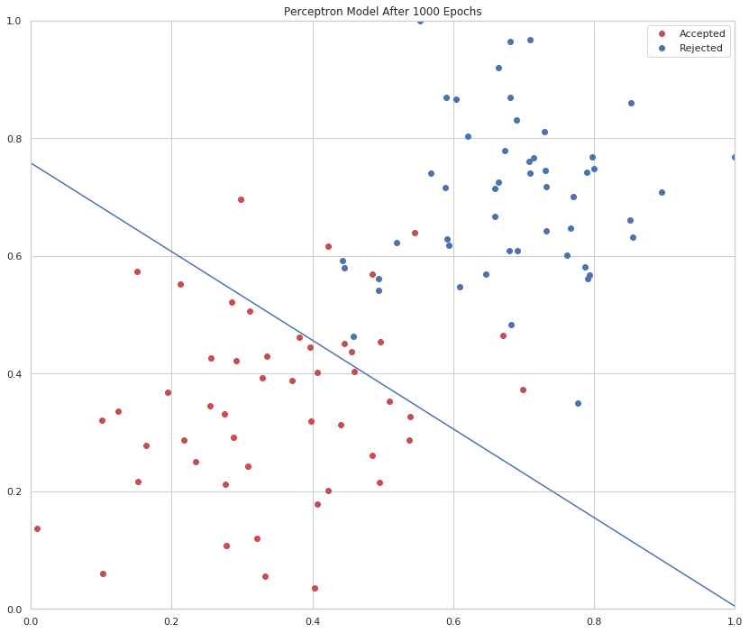
epochs = 1000
perceptron = Perceptron(x_train, y_train, epochs=epochs, verbosity=0)
perceptron.train()
print("Accuracy after {} epochs: {}".format(epochs, perceptron.accuracy))
figure, axe = pyplot.subplots(figsize=FIGURE_SIZE)
accepted = data[data.Label==1]
rejected = data[data.Label==0]
LIMITS = (0, 1)
axe.set_xlim(LIMITS)
axe.set_ylim(LIMITS)
axe.set_title("Perceptron Model After {} Epochs".format(epochs))
axe.plot(accepted.Test, accepted.Grades, 'ro', label="Accepted")
axe.plot(rejected.Test, rejected.Grades, "bo", label="Rejected")
axe.plot([0, 1], [perceptron.separator(0), perceptron.separator(1)])
legend = axe.legend()

model_separation.png

Perceptrons

Imports

From PyPi

from graphviz import Digraph
import matplotlib.pyplot as pyplot
import numpy
import pandas
import seaborn

Setup the Plotting

%matplotlib inline
seaborn.set(style="whitegrid")
FIGURE_SIZE = (14, 12)

What is a Perceptron?

A perceptron is a model based on the neuron that works as a linear classifier.

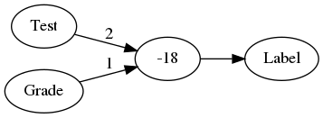
Our acceptance model from the previous post:

\[ 2x_1 + x_2 - 18 = 0 \]

Would be modeled by something like this.

graph = Digraph(comment="Perceptron", format="png")
graph.graph_attr["rankdir"] = "LR"
graph.node("a", "Test")
graph.node("b", "Grade")
graph.node("c", "-18")
graph.node("d", "Label")
graph.edge("a", "c", label="2")
graph.edge("b", "c", label="1")
graph.edge("c", "d")
graph.render("graphs/perceptron.dot")
graph

perceptron.dot.png

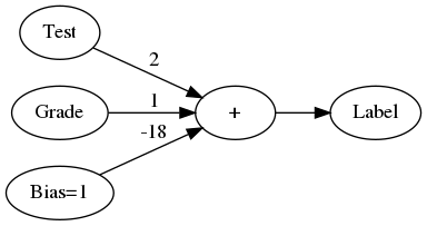
Where the weights on the edges of the graph are multiplied by the values from the input nodes and then added together with -18. The constant we add at the end is called a bias value, and an alternative way to notate it is to add an input node for it that always has a value of 1 for the input and -18 for the edge. This is equivalent to the previous graph but makes it a little more consistent.

graph = Digraph(comment="Perceptron 2", format="png")
graph.graph_attr["rankdir"] = "LR"
graph.node("a", "Test")
graph.node("b", "Grade")
graph.node("e", "Bias=1")
graph.node("c", "+")
graph.node("d", "Label")
graph.edge("a", "c", label="2")
graph.edge("b", "c", label="1")
graph.edge("e" , "c", label="-18")
graph.edge("c", "d")
graph.render("graphs/perceptron_2.dot")
graph

perceptron_2.dot.png

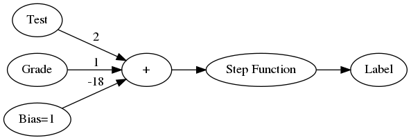
We can re-draw the graph to make it more explicit that there is a separate step-wise function to convert the score to a label, as well as use the more general notation of x and w.

graph = Digraph(comment="Perceptron 3", format="png")
graph.graph_attr["rankdir"] = "LR"
graph.node("a", "Test")
graph.node("b", "Grade")
graph.node("e", "Bias=1")
graph.node("c", "+")
graph.node("d", "Step Function")
graph.node("f", "Label")
graph.edge("a", "c", label="2")
graph.edge("b", "c", label="1")
graph.edge("e" , "c", label="-18")
graph.edge("c", "d")
graph.edge("d", "f")
graph.render("graphs/perceptron_3.dot")
graph

perceptron_3.dot.png

Why are these called neural networks?

The perceptron is modeled on a neuron in the brain which takes signal inputs and decides to fire (or not) based on these inputs.

Can perceptrons do logic?

The AND operator

Here's the truth table for the And operator.

Input 1 Input 2 Output
0 0 0
0 1 0
1 0 0
1 1 1

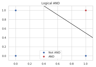
So how would you make a perceptron for this? Remember that the perceptron is a linear separator, so if you think if the two inputs as axes on the plane, you would fit a line that separates the outputs of 0 from the output of 1.

A Perceptron Class

class Perceptron:
    """Simple single perceptron

    Args:
     weight_x: weight for input x values
     weight_y: weight for input y values (x2)
     bias: bias scalar
    """
    def __init__(self, weight_x: float, weight_y: float, bias: float) -> None:
        self.weight_x = weight_x
        self.weight_y = weight_y
        self.bias = bias
        return

    def score(self, x: float, y: float) -> float:
        """calculate score for the inputs

       Args:
        x, y: inputs to the linear equation

       Returns:
        score: value representing which side of the line the point is
       """
        return self.weight_x * x + self.weight_y * y + self.bias

    def separator(self, x:float) -> float:
        """generates the values for the separation line

       Args: 
        x: the input value to generate the y-value for

       Returns:
        y: value for the plot given x
       """
        return -(self.weight_x * x + self.bias)/self.weight_y

    def update(self, weights: numpy.ndarray) -> None:
        """Updates the weights

       Args:
        weights: array of new weights (including bias)
       """
        self.weight_x = weights[0]
        self.weight_y = weights[1]
        self.bias = weights[2]
        return

    def __call__(self, x:float, y:float) -> int:
        """converts the score to a label

       This is the stepwise function

       Args:
        x, y: point values to check 

       Returns:
        label: 1 if right of the line, 0 otherwize
       """
        return int(self.score(x, y)>=0)

A Truth Table Printer

def truth_table(perceptron):
    binary = [0, 1]
    print("|Input 1|Input 2| Label|")
    print("|-+-+-|")
    for input_1 in binary:
        for input_2 in binary:
            output = perceptron(input_1, input_2)
            print(
                "|{}|{}|{}|".format(
                    input_1, input_2, output))
    return
perceptron_and = Perceptron(weight_x=1, weight_y=1, bias=-1.5)

So now here's the perceptron's truth table.

truth_table(perceptron_and)
Input 1 Input 2 Label
0 0 0
0 1 0
1 0 0
1 1 1
figure, axe = pyplot.subplots()
axe.set_xlim((-.1, 1.1))
axe.set_ylim((-.1, 1.1))
axe.plot([0,0,1], [0, 1, 0], "bo", label="Not AND")
axe.plot([0.4, 1.1], [perceptron_and.separator(0.4), perceptron_and.separator(1.1)], "k")
axe.plot([1], [1], "ro", label="AND")
axe.set_title("Logical AND")
legend = axe.legend()

perceptron_and.png

Perceptron OR

A similar thing can be done for the OR operator.

Input 1 Input 2 Output
0 0 0
0 1 1
1 0 1
1 1 1
perceptron_or = Perceptron(weight_x=1, weight_y=1, bias=-0.5)

And once again I'll check that the perceptron can replicate the truth table.

truth_table(perceptron_or)
Input 1 Input 2 Label
0 0 0
0 1 1
1 0 1
1 1 1
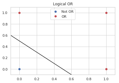
figure, axe = pyplot.subplots()
axe.plot([0], [0], "bo", label="Not OR")
axe.set_xlim((-.1, 1.1))
axe.set_ylim((-.1, 1.1))
axe.plot([-0.1, 0.8], [perceptron_or.separator(-0.1),
                       perceptron_or.separator(0.8)], "k")
axe.plot([0, 1, 1], [1, 0, 1], "ro", label="OR")
axe.set_title("Logical OR")
legend = axe.legend()

perceptron_or.png

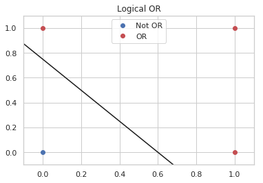
If you look at the plot you can see that the separator has to move lower, so, somewhat unintuitively your intercept (bias) should be less negative.

Or you should give more weight to the inputs.

perceptron_or_2 = Perceptron(weight_x=2.5, weight_y=2, bias=-1.5)

And here's the table generated with the same bias as the AND perceptron but with heavier weights.

truth_table(perceptron_or_2)
Input 1 Input 2 Label
0 0 0
0 1 1
1 0 1
1 1 1
figure, axe = pyplot.subplots()
axe.plot([0], [0], "bo", label="Not OR")
axe.set_xlim((-.1, 1.1))
axe.set_ylim((-.1, 1.1))
axe.plot([-0.1, 0.8], [perceptron_or_2.separator(-0.1),
                       perceptron_or_2.separator(0.8)], "k")
axe.plot([0, 1, 1], [1, 0, 1], "ro", label="OR")
axe.set_title("Logical OR")
legend = axe.legend()

perceptron_or_2.png

Seems to work okay.

NOT

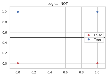
The NOT operation only looks at one input. To re-use our perceptron we can set the weights so it ignores the first input and negates the second.

Here's the Truth Table for NOT.

X NOT
0 1
1 0

So now we create a perceptron with an x-weight of 0.

perceptron_not = Perceptron(weight_x = 0, weight_y=-1, bias=0.5)

And see the output.

truth_table(perceptron_not)
Input 1 Input 2 Label
0 0 1
0 1 0
1 0 1
1 1 0

The table is overkill, since we only need to test two outputs, but it shows that even with the same inputs as the other perceptrons it can negate the second input.

figure, axe = pyplot.subplots()
axe.set_xlim([-.1, 1.1])
axe.set_ylim([-.1, 1.1])
axe.plot([0, 1], [0, 0], "ro", label="False")
axe.plot([0, 1], [1, 1], "bo", label="True")
axe.plot([-.1, 1.1], [perceptron_not.separator(-.1), 
                      perceptron_not.separator(1.1)], "k")
axe.set_title("Logical NOT")
legend = axe.legend()

perceptron_not.png

What about the XOR?

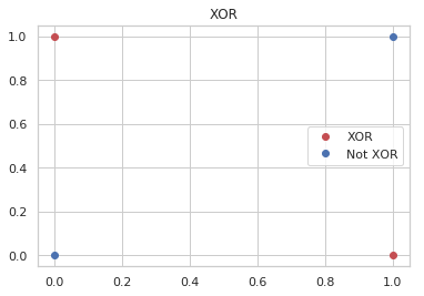
The XOR operator only returns True if one or the other input is True, not if both are True.

Input 1 Input 2 XOR
0 0 0
0 1 1
1 0 1
1 1 0
figure, axe = pyplot.subplots()
axe.set_title("XOR")
axe.plot([0, 1], [1, 0], "ro", label="XOR")
axe.plot([0, 1], [0, 1], "bo", label="Not XOR")
legend = axe.legend()

perceptron_xor.png

If you look at the plot you can see that a single straight line won't separate the blue and the red dots. The solution turns out to add a layers of perceptrons to make it work.

graph = Digraph(comment="Multilayer Perceptron", format="png")
graph.graph_attr['rankdir'] = "LR"
graph.node("a", " ")
graph.node("b", " ")
graph.node("c", "A")
graph.node("d", "B")
graph.node("e", "C")
graph.node("f", "AND")
graph.node("g", "XOR")
graph.edges(["ac", "ad", 'bc', 'bd', 'ce', 'ef', 'df', 'fg'])
graph.render("graphs/multilayer_perceptron.dot")
graph

multilayer_perceptron.dot.png

A, B, and C are OR, NOT and AND perceptrons, the key is to figure out which is which. The trick is to notice that AND is True when both are true, so we want B to to be 1 everytime there is at least one True and C to negate the one case when they're both True. So B is an OR, C is NOT and A is an AND (because and is True only when they're both True and C negates it).

graph = Digraph(comment="Multilayer Perceptron", format="png")
graph.graph_attr['rankdir'] = "LR"
graph.node("a", " ")
graph.node("b", " ")
graph.node("c", "AND 1")
graph.node("d", "OR")
graph.node("e", "NOT")
graph.node("f", "AND 2")
graph.node("g", "XOR")
graph.edges(["ac", "ad", 'bc', 'bd', 'ce', 'ef', 'df', 'fg'])
graph.render("graphs/multilayer_perceptron_2.dot")
graph

multilayer_perceptron_2.dot.png

Input 1 Input 2 AND 1 NOT OR AND 2
0 0 0 1 0 0
0 1 0 1 1 1
1 0 0 1 1 1
1 1 1 0 1 0

It's not the clearest table, but AND 1 and OR both take the original inputs, then NOT negates AND 1 and the output of NOT and OR feed into AND 2 which puts out our exclusive or.

Here's what happens when we use the perceptrons we created earlier to generate the same table.

inputs = [[0, 0],
          [0, 1],
          [1, 0],
          [1, 1]]

print("| Input 1 | Input 2 | AND 1 | NOT | OR | XOR |")
print("|---------+---------+-------+-----+----+-------|")
row = "|" + "{}|" * 6
for (x, y) in inputs:
    and_1 = perceptron_and(x, y)
    nand = perceptron_not(0, and_1)
    or_1 = perceptron_or(x, y)
    xor = perceptron_and(nand, or_1)
    print(row.format(x, y, and_1, nand, or_1, xor))
Input 1 Input 2 AND 1 NOT OR XOR
0 0 0 1 0 0
0 1 0 1 1 1
1 0 0 1 1 1
1 1 1 0 1 0

Looks right.

Nand

that the combination or AND and NOT is a NAND operator so you could simplify the diagram a little back to just two layers.

graph = Digraph(comment="Two-Layer XOR Perceptron", format="png")
graph.graph_attr['rankdir'] = "LR"
graph.node("a", " ")
graph.node("b", " ")
graph.node("c", "NAND")
graph.node("d", "OR")
graph.node("f", "AND")
graph.node("g", "XOR")
graph.edges(["ac", "ad", 'bc', 'bd', "cf", 'df', 'fg'])
graph.render("graphs/two_layer_xor.dot")
graph

two_layer_xor.dot.png

That's a lot of work to get an XOR, how are we going to classify images like this?

This isn't about image classification, but we probably should note that you normally wouldn't try and figure out the parameters by hand, the perceptron can tune itself. The way it does this is by picking some initial random values and then it repeatedly tests how well it did and adjusts the weights.

How does it adjust the weights?

This is what's called "the Perceptron Trick". It basically forms a vector for each of the misclassified points \((x_1, x_2, 1)\) and subtracts it from the weights \((w_1, w_2, b)\) if the score was on the positive side and adds to it if the score was on the negative side. It then repeats this for each of the misclassified points. Since we have multiple points we don't want it to just make these huge jumps, so the misclassified points vector is multiplied by some fraction (called the learning rate) so that the changes are small. Once it has the new weights it then tests itself again and makes another adjustment.

Question

If the original line was \(3x_1 + 4x_2 - 10 = 0\), and the learning rate was set to 0.1, how many adjustments would you have to make to reach the point (1, 1)?

x, y = 1, 1
weights = numpy.array([3, 4, -10])
learning_rate = 0.1
adjustment = numpy.ones(3) * learning_rate
output = 0
adjustments = 0
perceptron = Perceptron(weights[0], weights[1], weights[2])
while True:
    output = perceptron.score(x, y)
    if output >= 0:
        break
    print(output)
    adjustments += 1
    direction = 1 if output < 0 else -1
    weights = weights + direction * adjustment
    perceptron.update(weights)
print("Final Output: {}".format(output))
print(print("Adjustments: {}".format(adjustments)))
-3
-2.700000000000001
-2.4000000000000012
-2.1000000000000014
-1.8000000000000025
-1.5000000000000036
-1.2000000000000028
-0.9000000000000039
-0.600000000000005
-0.30000000000000604
-7.105427357601002e-15
Final Output: 0.29999999999999183
Adjustments: 11
None

I came up with 11 adjustments but Udacity says 10… Close enough, I guess.

Introduction to Neural Networks

Imports

From ipython

from typing import Union

From Pypi

from graphviz import Digraph
import matplotlib.pyplot as pyplot
import numpy
import pandas
import seaborn

This Project

from neurotic.tangles.data_paths import DataPath

Setup the Plotting

%matplotlib inline
seaborn.set(style="whitegrid")
FIGURE_SIZE = (14, 12)

Some Types

Identifier = Union[str, int]

Introduction

These are notes on the series Introduction to Neural Networks taught by Luis Serrano as part of Udacity's Deep Learning Nan Degree.

What are Neural Networks

Neural Networks are algorithms loosely based on the neurons in the brain. Although biologically inspired, in many ways what they do can be viewed as linear separation. But as the complexity of the network builds, this simple idea can produce outcomes that look much more complicated.

Classification Problems

Example: College Admissions

You have a set of test scores and grades for students who applied to a university, as well as whether they were accepted or rejected. For example:

Student Test Grades Accepted
1 9/10 8/10 Yes
2 3/10 4/10 No

You have a new student 3 and you're wondering if he will likely get accepted.

Student Test Grades
3 7/10 6/10

Linear Boundaries

We're going to make our prediction using a linear classifier that decides if the student is above or below a line that separates the accepted and rejected students. A boundary line is defined by inputs (x), weights (w), and an intercept (b). For the two-dimensional case the equation would be this.

\[ w_1 x_1 + w_2 x_2 + b = 0 \]

For our example the boundary line turns out to be:

\[ 2x_1 + x_2 - 18 = 0 \]

or to use our naming scheme.

\[ 2 \times \textit{Test} + \textit{Grades} - 18 = \textit{Score} \]

Once we have the score our prediction will be based on the sign of the score. If it is positive we will predict an acceptance and if it is negative, we will predict a rejection. If a student has a score if 0 that means he or she is on the line, so to make it a binary classification we will say that we will accept the student if the score is zero as well.

A More Formal Version

Our equation for our line is composed of two vectors that output a number which we will label either 1 (accepted) or 0 (rejected) based on the output.

Our original equation:

\[ w_x x_1 + w_2 x_2 + b = 0 \]

Can be re-written using vectors.

\[ Wx + b = 0\\ W = (w_1, w_2)\\ x = (x_1, x_2)\\ \]

And our labels for the outcomes are in this set. \[ y \in \{0, 1\}\\ \]

Our prediction is a stepwise function that we hope will match the true label.

\[ \hat{y} = \begin{cases} 1 \text{ if } Wx + b \geq 0\\ 0 \text{ if } Wx + b \lt 0 \end{cases} \]

What would our score be for Student 3?

class Student:
    """Holds the student's info

    Args:
     name: identifier for the student
     test: score on the test
     grades: student's grade value (average?)
    """
    def __init__(self, name: Identifier, test: float, grades: float) -> None:
        self.name = name
        self.test = test
        self.grades = grades
        return

    def __str__(self) -> str:
        """something to identify the student"""
        return "Student {}".format(self.name)
class Score:
    """Calculate the score for our student

    Args:
     student: a Student
     test_weight: the weight for the test score     
     bias: the bias value
    """
    def __init__(self, student: Student,
                 test_weight: float=2, bias: float=-18) -> None:
        self.student = student
        self.test_weight = test_weight
        self.bias = bias
        self._score = None
        self._label = None
        self._outcome = None
        return

    @property
    def score(self) -> float:
        """The calculated score for the student"""
        if self._score is None:
            self._score = (self.test_weight * self.student.test
                           + self.student.grades
                           + self.bias)
        return self._score

    @property
    def label(self) -> int:
        """A classification for this score (0|1)"""
        if self._label is None:
            self._label = 1 if self.score >= 0 else 0
        return self._label

    @property
    def outcome(self) -> str:
        """whether the student was accepted or rejected"""
        if self._outcome is None:
            self._outcome = "Accepted" if self.label == 1 else "Rejected"
        return self._outcome

    def __str__(self) -> str:
        """Pretty printed outcomes (an org-table)"""
        output =  "||Value|\n"
        output += "|-+-|\n"
        output += "|Score|{:.2f}|\n".format(self.score)
        output += "|Label|{}|\n".format(self.label)
        output += "|Prediction|{}|".format(self.outcome)
        return output
student_3 = Student(name=3, test=7, grades=6)
score = Score(student_3)
print(str(score))
  Value
Score 2.00
Label 1
Prediction Accepted

He got a positive score so we predict that he will get in.

Plot the Separation

To plot the separation we have to re-write our equation so the y (called Grades) is on one side of the equation.

\[ w_1 x_1 + w_2 x_2 + b = 0\\ w_2 x_2 = -w_1 x_1 - b\\ \textit{grade} = -2\textit{test} + 18\\ \]

def separation(x: float, slope: float=-2, y_intercept: float=18) -> float:
    """gives the y-value for the separation line

    Args:
     x: input value
     slope: slope value
     y_intercept: y-intercept value

    Returns:
     y: value on the linear separation line
    """
    return slope * x + y_intercept
figure, axe = pyplot.subplots(figsize=FIGURE_SIZE)
limit = (0, 10)
axe.set_xlim(limit)
axe.set_ylim(limit)
axe.set_title(str(student_3))
grades = [separation(0), separation(10)]
axe.plot(student_3.test, student_3.grades, 'o', label=str(student_3))
axe.set_xlabel("Test")
axe.set_ylabel("Grades")
lines = axe.plot(limit, grades)
legend = axe.legend()

score_1.png

If the test was weighted 1.5 instead of 2, would our student still have gotten in?

TEST_WEIGHT = 1.5
score = Score(student_3, test_weight=TEST_WEIGHT)
print(str(score))
  Value
Score -1.50
Label 0
Prediction Rejected
SLOPE = -TEST_WEIGHT
figure, axe = pyplot.subplots(figsize=FIGURE_SIZE)
limit = (0, 10)
axe.set_xlim(limit)
axe.set_ylim(limit)
axe.set_title("{} with Test Weight {}".format(student_3, TEST_WEIGHT))
grades = [separation(0, slope=SLOPE), separation(10, slope=SLOPE)]
axe.plot(student_3.test, student_3.grades, 'o', label=str(student_3))
axe.set_xlabel("Test")
axe.set_ylabel("Grades")
lines = axe.plot(limit, grades)
legend = axe.legend()

score_2.png

The student is to the left of the separation and so won't get in, as we found earlier.

What about more variables?

For every variable you add you add an extra dimension. So if you add one more variable, instead of a line our separator will be a plane.

\[ w_1 x_1 + w_2 x_2 + w_3 x_3 + b = 0 \]

But when you use vector notation it will look the same.

\[ Wx + b = 0 \hat{y} = \begin{cases} 1 \text{ if } Wx + b \geq 0\\ 0 \text{ if } Wx + b \lt 0 \end{cases} \]

This will be true no matter how many variable (dimensions) you add.

Question

You have a table with n columns representing features to evaluate students and each row is a student. What would be the shapes of the vectors?

W x b
1 x n n x 1 1 x 1

Our output is a single value, so the rows for weights and columns for inputs should be 1, and b is just a scalar.

NumPy Practice One

Imports

import numpy

Prepare Inputs

def prepare_inputs(inputs):
    """transforms inputs and does some math

    Creates a 2-dimensional ndarray from the given 1-dimensional list
     and assigns  it to input_array

    Finds the minimum value in the input array and subtracts that
     value from all the elements of input_array.

    Finds the maximum value in inputs_minus_min and divides
     all of the values in inputs_minus_min by the maximum value.

    Args:
     inputs: one-dimensional list

    Returns:
     tuple: transposed inputs, inputs-minus-min, inputs-minus-min scaled by max
    """
    input_array = numpy.array([inputs])
    inputs_minus_min = input_array - input_array.min()
    inputs_div_max = inputs_minus_min/inputs_minus_min.max()
    return input_array, inputs_minus_min, inputs_div_max
inputs = [1, 2, 3]
transposed, less_min, divided_by_max = prepare_inputs(inputs)
print(transposed)
expected = numpy.array([0, 1, 2])
assert all(expected == less_min[0,:])
print(less_min)
assert all(expected/2 == divided_by_max[0, :])
print(divided_by_max)
[[1 2 3]]
[[0 1 2]]
[[0.  0.5 1. ]]

Multiply Inputs

def multiply_inputs(m1, m2):
    """Multiplies matrices

    Args:
     m1, m2: matrices to multiply

    Returns:
     matrix product or False if shapes are wrong
    """
    product = False
    okay, swap = m1.shape[1] == m2.shape[0], m1.shape[0] == m2.shape[1]
    if any((okay, swap)):
        product = m1.dot(m2) if okay else m2.dot(m1)
    return product
ROW, COLUMN = 0, 1
m_1 = numpy.array([1, 2, 3, 4, 5, 6]).reshape((2, 3))
m_2 = numpy.array([6, 5, 4, 3, 2, 1]).reshape((2, 3))
m_3 = m_2.reshape((3, 2))
m_4 = numpy.arange(12).reshape(6, 2)
print(m_3.shape)

print("{} x {}".format(m_1.shape, m_2.shape))
product = multiply_inputs(m_1, m_2)
assert not product
print(product)

print("\n{} x {}".format(m_1.shape, m_3.shape))
product = multiply_inputs(m_1, m_3)
assert product.shape == (m_1.shape[ROW], m_3.shape[COLUMN])
print(product)
print(product.shape)

print("\n{} x {}".format(m_1.shape, m_4.shape))
product = multiply_inputs(m_1, m_4)
assert product.shape == (m_4.shape[ROW], m_1.shape[COLUMN])
print(product)
print(product.shape)
(3, 2)
(2, 3) x (2, 3)
False

(2, 3) x (3, 2)
[[20 14]
 [56 41]]
(2, 2)

(2, 3) x (6, 2)
[[ 4  5  6]
 [14 19 24]
 [24 33 42]
 [34 47 60]
 [44 61 78]
 [54 75 96]]
(6, 3)

Find the mean

def find_mean(values):
    """Find the mean value

    Args:
     values: list of numeric values
    Returns:
     the average of the values in the given Python list
    """
    return numpy.array(values).mean()
inputs = [[1, 5, 9]]
outputs = find_mean(inputs)
print(outputs)
assert abs(sum(inputs[0])/len(inputs[0]) - outputs) < 0.1**5
5.0

More Outputs

input_array, inputs_minus_min, inputs_div_max = prepare_inputs([-1,2,7])
print("Input as Array: {}".format(input_array))
print("Input minus min: {}".format(inputs_minus_min))
print("Input  Array: {}".format(inputs_div_max))

print("Multiply 1:\n{}".format(multiply_inputs(numpy.array([[1,2,3],[4,5,6]]), numpy.array([[1],[2],[3],[4]]))))
print("Multiply 2:\n{}".format(multiply_inputs(numpy.array([[1,2,3],[4,5,6]]), numpy.array([[1],[2],[3]]))))
print("Multiply 3:\n{}".format(multiply_inputs(numpy.array([[1,2,3],[4,5,6]]), numpy.array([[1,2]]))))

print("Mean == {}".format(find_mean([1,3,4])))
Input as Array: [[-1  2  7]]
Input minus min: [[0 3 8]]
Input  Array: [[0.    0.375 1.   ]]
Multiply 1:
False
Multiply 2:
[[14]
 [32]]
Multiply 3:
[[ 9 12 15]]
Mean == 2.6666666666666665

How do you handle multiple inputs and outputs?

Beginning

Imports

From Python

 from functools import partial
 from pathlib import Path
 from typing import List

From PyPi

from graphviz import Digraph
from tabulate import tabulate

import holoviews
import numpy
import pandas

Set Up

Table Printer

TABLE = partial(tabulate, tablefmt="orgtbl", headers="keys")

Plotting

SLUG = "how-do-you-handle-multiple-inputs-and-outputs"
ROOT = "../../../files/posts/grokking/03_forward_propagation/"
OUTPUT_PATH = Path(ROOT)/SLUG

Embed = partial(EmbedHoloviews, folder_path=OUTPUT_PATH)

Some Types

Vector = List[float]
Matrix = List[Vector]

What is this?

This is a continuation of my notes on Chapter Three of "Grokking Deep Learning". In the previous post we looked at a simple neural network with one input and three outputs. Here we'll look at handling multiple inputs and outputs.

Middle

So how do you handle multiple inputs and outputs?

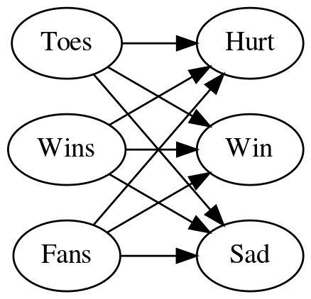
You create a network that has a node for each of the inputs and each input node has an output to each of the outputs. Here's the matrix representation of the network we're going to use.

data = pandas.DataFrame(
    dict(
        source=["Toes"] * 3 + ["Wins"] * 3 + ["Fans"] * 3,
        target=["Hurt", "Win", "Sad"] * 3,
        edge = [0.1, 0.1, 0, 0.1, 0.2, 1.3, -0.3, 0.0, 0.1]))
print(TABLE(data, showindex=False))
source target edge
Toes Hurt 0.1
Toes Win 0.1
Toes Sad 0
Wins Hurt 0.1
Wins Win 0.2
Wins Sad 1.3
Fans Hurt -0.3
Fans Win 0
Fans Sad 0.1

network.dot.png

Adding the weights to the diagram made it hard to read so here's a table version of the weights for the edges.

edges = data.pivot(index="target", columns="source", values="edge")
edges.columns.name = None
edges.index.name = None
print(TABLE(edges))
  Fans Toes Wins
Hurt -0.3 0.1 0.1
Sad 0.1 0 1.3
Win 0 0.1 0.2

Okay, but how do you build that network?

It's basically the same as with one output except you repeat for each node - for each node you calculate the weighted sum (dot product) of the inputs.

Dot Product

def weighted_sum(inputs, weights):
    """Calculates the weighted sum of the inputs

    Args:

    """
    assert len(inputs) == len(weights)
    return sum((inputs[index] * weights[index] for index in range(len(inputs))))

Vector-Matrix Multiplication

We'll take the inputs as a vector of length three since we have three features and the weights as a matrix of three rows and three columns and then multiply the inputs by each of the rows of weights using the dot product to get our three outputs.

  • for each output take the dot product of the weights of its inputs and the input vector
def vector_matrix_multiplication(vector: Vector, matrix: Matrix) -> Vector:
    """takes the dot product of each row in the matrix and the vector

    Args:
     vector: the inputs to the network
     matrix: the weights

    Returns:
     outputs: the network's outputs
    """
    vector_length = len(vector)
    assert vector_length == len(matrix)
    return [weighted_sum(vector, matrix[output])
            for output in range(vector_length)]

To test it out I'll convert the weights to a matrix (list of lists).

weights = edges.values

Now we'll create a team that averages 8.5 toes per player, has won 65 percent of its games and has 1.2 million fans. Note that we have to match the column order of our edge data-frame.

TOES = 8.5
WINS = 0.65
FANS = 1.2
inputs = [FANS, TOES, WINS]

What does it predict? The output of our function will be a vector with the outputs in the order of the rows in our edge-matrix.

outputs = vector_matrix_multiplication(inputs, weights)
HURT = 0.555
SAD = 0.965
WIN = 0.98
expected_outputs = [HURT, SAD, WIN]
tolerance = 0.1**5
expected_actual = zip(expected_outputs, outputs)
names = "Hurt Sad Win".split()
print("| Node| Value|")
print("|-+-|")
for index, (expected, actual) in enumerate(expected_actual):
    print(f"|{names[index]}|{actual:.3f}")
    assert abs(actual - expected) < tolerance,\
            "Expected: {} Actual: {} Difference: {}".format(expected,
                                                            actual,
                                                            expected-actual)
Node Value
Hurt 0.555
Sad 0.965
Win 0.980

So we are predicting that they have a 98% chance of winning and a 97% chance of being sad? I guess the fans have emotional problems outside of sports.

The Pandas Way

predictions = edges.dot(inputs)
print(TABLE(predictions.reset_index().rename(
    columns={"index": "Node", 0: "Value"}), showindex=False))
Node Value
Hurt 0.555
Sad 0.965
Win 0.98

Ending

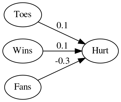
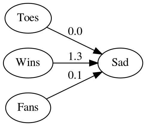
So, like we saw previously that finding the charge for a neuron is just vector math and making a network of neurons doesn't really change that, instead of doing it all as one matrix we could have taken each of our output nodes and treated them as a separate vector that we used to take the dot product:

print("|Node | Value|")
print("|-+-|")
for node in edges.index:
    print(f"|{node} |{edges.loc[node].dot(inputs): 0.3f}|")
Node Value
Hurt 0.555
Sad 0.965
Win 0.980

Which is like going back to our single neuron case for each output.

hurt_neuron.dot.png

Sad_neuron.dot.png

Win_neuron.dot.png

But by stacking them in a matrix it becomes easier to work with them as the network gets larger.

How do you handle multiple outputs?

Preliminaries

Imports

From Python

 from pathlib import Path
 from typing import List

From PyPi

 from graphviz import Digraph
 import numpy

Set Up

The Output Folder

This is where to put rendered images.

PATH = Path("../../../files/posts/grokking/03_forward_propagation/how-do-you-handle-multiple-outputs/")

Data Types

Vector = List[float]

Beginning

What is this?

This is a continuation of my notes on Chapter Three of "Grokking Deep Learning". In the previous post we looked at a simple neural network with three inputs and one output. Here we'll look at handling multiple outputs.

How do you handle one input and multiple outputs?

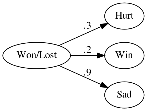
Suppose instead of using multiple inputs to predict an outcome (like winning) you instead had a single input and multiple outputs (like what percentage feels sad, or indifferent based on whether you won or lost as well as whether you will win). You could create a network to represent it something like this.

graph = Digraph(comment="Feelings Model", format="png", graph_attr={"rankdir": "LR", "dpi": "200"})
graph.node("A", "Won/Lost")
graph.node("B", "Hurt")
graph.node("C", "Win")
graph.node("D", "Sad")
graph.edge("A", "B", label=".3" )
graph.edge("A", "C", label=".2" )
graph.edge("A", "D", label=".9" )
graph.render(PATH/"feelings_model.dot")
graph

feelings_model.dot.png

How do you implement this?

In this case the outputs are simply the (single) input times the weight of the output, so while the single output was the dot-product of the inputs and the weights, this, the multiple output case, is an elementwise multiplication of the input and the weights.

def elementwise_multiplication(scalar: float, weights: Vector) -> Vector:
    """multiplies the value against each of the weights

    Returns:
     output: scalar times each of the weights as a list
    """
    return [scalar * weights[index] for index in range(len(weights))]

In Action

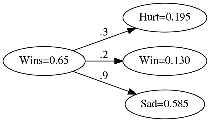
Here's some sample values that we can use to see what this network gives us. Our input is the fraction of the games won up to a given week and our outputs are the fraction of players that are hurt, the probability that they won or lost, and whether the players are happy or sad.

labels = "Hurt Win Sad".split()
weights = [0.3, 0.2, 0.9]
fraction_of_wins = [0.65, 0.8, 0.8, 0.9]

These are the probabilities of a fan feeling a certain way the first week.

wins = fraction_of_wins[0]
expected = [0.195, 0.13, 0.585]
actual = elementwise_multiplication(wins, weights)
tolerance = 0.1**5
for index, item in enumerate(actual):
    assert abs(expected[index] - item) < tolerance

graph = Digraph(comment="Feelings Model", format="png", graph_attr={"rankdir": "LR", "dpi": "200"})
graph.node("A", f"Wins={wins}")
graph.node("B", f"Hurt={actual[0]:.3f}")
graph.node("C", f"Win={actual[1]:.3f}")
graph.node("D", f"Sad={actual[2]:.3f}")
graph.edge("A", "B", label=".3" )
graph.edge("A", "C", label=".2" )
graph.edge("A", "D", label=".9" )
graph.render(PATH/"feelings_model_with_output.dot")
print("[[file:feelings_model_with_output.dot.png]]")

feelings_model_with_output.dot.png

How would you do this with numpy?

Since this is just element-wise multiplication, all you have to do is create an array and then multiply it by the scalar input.

vector_weights = numpy.array(weights)
actual = vector_weights * wins
vector_expected = numpy.array(expected)
numpy.testing.assert_allclose(actual, expected)

graph = Digraph(comment="Feelings Model", format="png", graph_attr={"rankdir": "LR", "dpi": "200"})
graph.node("A", f"Wins={wins}")
graph.node("B", f"Hurt={actual[0]:.3f}")
graph.node("C", f"Win={actual[1]:.3f}")
graph.node("D", f"Sad={actual[2]:.3f}")
graph.edge("A", "B", label=".3" )
graph.edge("A", "C", label=".2" )
graph.edge("A", "D", label=".9" )
graph.render(PATH/"numpy_feelings_model_with_output.dot")
print("[[file:numpy_feelings_model_with_output.dot.png]]")

numpy_feelings_model_with_output.dot.png

Pytorch?

Like numpy, pytorch uses the multiplication operator for element-wise multiplication.

device = torch.device("cuda") if torch.cuda.is_available() else torch.device("cpu")
weights_vector = torch.tensor(weights, device=device)
actual = (weights_vector * wins).tolist()
numpy.testing.assert_allclose(actual, expected)

graph = Digraph(comment="Feelings Model", format="png", graph_attr={"rankdir": "LR", "dpi": "200"})
graph.node("A", f"Wins={wins}")
graph.node("B", f"Hurt={actual[0]:.3f}")
graph.node("C", f"Win={actual[1]:.3f}")
graph.node("D", f"Sad={actual[2]:.3f}")
graph.edge("A", "B", label=".3" )
graph.edge("A", "C", label=".2" )
graph.edge("A", "D", label=".9" )
graph.render(PATH/"pytorch_feelings_model_with_output.dot")
print("[[file:pytorch_feelings_model_with_output.dot.png]]")

pytorch_feelings_model_with_output.dot.png

End

So that's it for handling multiple outputs from a node to multiple nodes. As with the many inputs to one node what you're really doing is vector math, when reducing from many to one you use the dot product and when going from one to many you use scalar multiplication.

How Do Neurons Work?

Beginning

Imports

Some if this is needed to draw the network so I'm putting all the imports first.

From Python

 from functools import partial
 from pathlib import Path
 from typing import List

From PyPi

from graphviz import Digraph
import holoviews
import hvplot.pandas
import numpy
import pandas
import torch

Others

from graeae import EmbedHoloviews

What is this about?

These are notes on Chapter Three of "Grokking Deep Learning". It is an explanation of how neural networks perform the first step of training the model - making predictions - illustrated with a single neuron. Predicting might seem like a step for after you finish training the model, but in order to correct the model you have to first make predictions to see how well it is doing. We'll look at a model that predicts whether a team will win a game based on a single feature (the average number of toes on the team).

Heres' the network.

SLUG = "how-do-neural-networks-work/"
PATH = Path("../../../files/posts/grokking/03_forward_propagation/")/SLUG
graph = Digraph(comment="Toes Model", format="png",
                graph_attr={"rankdir": "LR", "dpi": "200"})
graph.node("A", "Toes")
graph.node("B", "Win")
graph.edge("A", "B", label="w=0.1")
graph.render(PATH/"toes_model_1.dot")
graph

toes_model_1.dot.png

Although we're calling it a network we're really creating only the first building block for a single neuron. A neuron works by doing three basic things:

  1. It receives signals from other neurons (over dendrites, the inputs to the neuron)
  2. It aggregates the signals within the cell-body (soma) of the neuron
  3. If the cell voltage crosses a threshold then it fires a signal out across its axon

We can kind of say there's an implied axon to our network, it just isn't shown, and we can read the Toes node as either another neuron and the edge between it and the Win node is a synapse (Greek for conjunction) which contains an axon coming out of Toes that joins the dendrite going into Win), giving us a network of two nodes, but what we are missing is the test to see if the cell's charge exceeds a threshold. That will come later.

Set Up

Plotting

Embed = partial(
    EmbedHoloviews,
    folder_path=PATH)

holoviews.opts(width=1000, height=800)

Types

This is for type-hinting.

Numbers = List[float]

Middle

What is the simplest neural network we can create to make this prediction?

Our Network

toes_model_1.dot.png

Our network represents two neurons with a synapse between them. The dendrite leading into the Win neuron has a certain weight representing how much of the input signal (average number of toes) can get across it to the Win neuron - the higher the weight, the more signal it contributes to our Win neuron deciding whether to fire or not (once we add a threshold). In this case we have an arbitrary weight of 0.1. The input to the Win neuron is just the weight of the dendrite times the output of the Toes neuron.

In the book Grokking Deep Learning Andrew Trask uses the analogy of the weights being like the knob on a machine that turns the volume up and down (I don't think he says volume, but it's the same idea). This is something that I seem to recall seeing in books describing the coefficients for linear regression - every variable you add gives you another knob to tune, but since the more common analogy is to think of modeling artificial neurons in the brain, it might be better to think of the weights as the thickness of the dendrite.

 def one_neuron(toes: float, weight: float=0.1) -> float:
     """This is a model to predict whether a team will win

     Args:
      toes: Average number of toes on the team
      weight: how much to weight to give to the toes

     Returns:
      prediction: our guess as to the probability that they will win
     """
     return toes * weight

Some Predictions

We can test out what our model thinks with some test values.

 average_toes = [8.5, 9, 9.5, 10]
 predictions = [one_neuron(toe) for toe in average_toes]
 print("| Toes | Probability of Winning (%)|")
 print("|-+-|")
 for index, toes in enumerate(average_toes):
     prediction = predictions[index] * 100
     print(f"| {toes} | {prediction:.0f} % |")
Toes Probability of Winning (%)
8.5 85 %
9 90 %
9.5 95 %
10 100 %
 data = pandas.DataFrame({"Average Toes": average_toes,
                          "Probability of Winning": predictions})
 plot = data.hvplot(x="Average Toes", y="Probability of Winning").opts(
     width=1000, height=800, title="Toe Model")
 Embed(plot=plot, file_name="toes_only_predictions")()

Figure Missing

As you can see, it's just a straight line. If we think in terms of the familiar \(y=mx + b\), our model is the equivalent of:

\[ probability = 0.1 \times toes \]

Where \(b=0\). So every toe contributes 10% to our prediction.

What does knowledge and information mean in our neural network?

The neural network stores its knowledge as weights and when given information (input) it converts them to a prediction (output).

What kind of memory does a neuron have?

A neuron stores what its learned (long-term memory) as the weight on the edge(s). The neuron as we've implemented it doesn't have any short-term memory, it can only consider one input at a time and "forgets" the previous input that it got. To have short-term memory you need to employ a different method that uses multiple inputs at the same time.

So weights are memory, but what is it memorizing?

Since the neuron represents one feature (average toes) the weight is how important this feature is to the outcome (winning). If you have multiple features, the weights turn up or down the volume for each of the features (thus the knob analogy).

So, how do you handle multiple inputs?

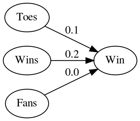
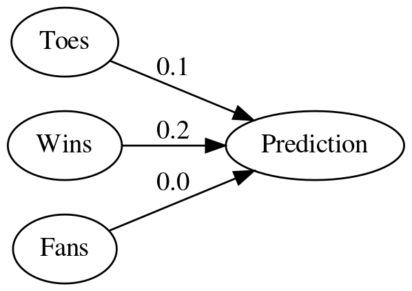
If you have multiple inputs then your prediction is the sum of the individual inputs times their weights.

 graph = Digraph(comment="Three Nodes", format="png",
                 graph_attr={"rankdir": "LR", "dpi": "200"})
 graph.node("A", "Toes")
 graph.node("B", "Wins")
 graph.node("C", "Fans")
 graph.node("D", "Prediction")
 graph.edge("A", "D", label="0.1")
 graph.edge("B", "D", label="0.2")
 graph.edge("C", "D", label="0.0")
 graph.render(PATH/"three_nodes.dot")

three_nodes.dot.png

Here we've added two more input neurons - Wins is the fraction of games played that the team won and Fans is the number of fans the team has (in millions).

Weighted Sum

Since we have three nodes we need to return the sum of the weights and inputs. If we think of the weights and inputs as vectorns then this is their dot-product.

 def weighted_sum(inputs: Numbers, weights: Numbers) -> float:
     """calculates the sum of the products

     Args:
      inputs: list of input data
      weights: list of weights for the inputs

     Returns:
      sum: the sum of the product of the weights and inputs
     """
     assert len(inputs) == len(weights)
     return sum((inputs[item] * weights[item] for item in range(len(inputs))))

The Node

Right now this next function is just an alias for the weighted_sum but eventually we'll be doing more with it.

 def network(inputs: Numbers, weights:Numbers) -> float:
     """Makes a prediction based on the inputs and weights"""
     return weighted_sum(inputs, weights)

Some Inputs

We have some data collected about our team over four games.

Variable Description
toes average number of toes the members have at game-time
record fraction of games won
fans Millions of fans that watched
 toes = [8.5, 9.5, 9.9, 9.0]
 record = [0.65, 0.8, 0.8, 0.9]
 fans = [1.2, 1.3, 0.5, 1.0]

Each entry in the vectors is the value that was true just before each game. This makes the first record entry sort of non-sensical, but it's just an illustration.

 weights = [0.1, 0.2, 0.0]

The weights correspond to (toes, record, fans) for each game so we weight the win-loss record the most and fans not at all. Our for game i (so 0 if it's the first game), our prediction will be calculated as:

\begin{align} prediction_i &= toes_i \times weights_0 + record_i \times weights_1 + fans_i \times weights_2\\ &= (0.1) toes_i + (0.2) record_i + (0) fans_i\\ \end{align}
print("|Game|Prediction|")
print("|-+-|")

predictions = [
    network([toes[game], record[game], fans[game]], weights)
               for game in range(len(toes))]
assert abs(predictions[0] - 0.98) < 0.1**5

for game, prediction in enumerate(predictions):
    print(f"|{game + 1}|{prediction:.2f}")
Game Prediction
1 0.98
2 1.11
3 1.15
4 1.08

With the exception of game one we're predicting that the combination of toes and previous wins make the win pretty much inevitable. We should also note that the highestt prediction went to the third game which was the game with the highest number of average toes. Even though we weighted the win-loss record higher, the values being passed in are much greater for the toes than for the win-loss record.

 data = pandas.DataFrame({"toes": toes, "record": record,
                          "prediction": predictions})
 data = data.sort_values(by="toes")
 prediction_plot = data.hvplot(x="toes", y="prediction")
 other = data.hvplot(x="toes", y="record")
 plot = (prediction_plot * other).opts(
     title="Toes vs Record & Prediction",
     width=1000,
     height=800,
 )

 Embed(plot=plot, file_name="toes_vs_record")()

Figure Missing

Looking at the plot you can see that the probability keeps climbing with the number of toes and the peak record (9 toes, 90% wins) is canceled out by the fact that it occurs with a team with fewer toes than the peak of 9.9 toes.

How would you do this with numpy?

Although we used for-loops to calculate the predictions, we can view each of the inputs as a vector and the weights as a vector and then the prediction becomes the dot product of the inputs and the weights, so we can use numpy's dot method to calculate it for us.

 print("|Game|Prediction|")
 print("|-+-|")

 network = numpy.array([toes, record, fans])
 predictions = network.T.dot(weights)
 assert abs(predictions[0] - 0.98) < 0.1**5

 for game, prediction in enumerate(predictions):
     print(f"|{game + 1}|{prediction:.2f}|")
Game Prediction
1 0.98
2 1.11
3 1.15
4 1.08

What about pytorch

Pytorch can act like numpy working on the GPU, making the calculations faster, but the syntax is a little different (and it uses matmul instead of dot).

print("|Game|Prediction|")
print("|-+-|")

device = torch.device("cuda") if torch.cuda.is_available() else torch.device("cpu")
inputs = torch.tensor([toes, record, fans], device=device)
weights_vector = torch.tensor(weights, device=device)
predictions = inputs.T.matmul(weights_vector).tolist()
for game, prediction in enumerate(predictions):
    print(f"|{game + 1}|{prediction:.2f}|")
Game Prediction
1 0.98
2 1.11
3 1.15
4 1.08

Note: In this simple case the pytorch version can be much slower than the numpy version - sometimes "optimization" isn't really optimal.

End

The main takeaway from this is that a neuron is takes the weighted sum of its input in order to build its internal value (its charge) and the weighted sum is in turn the dot product of the weight vector and the input vector.

Sources

  • [GDL] Trask AW. Grokking Deep Learning. Shelter Island: Manning; 2019. 309 p.
  • [DLI] Krohn J. Deep Learning Illustrated: a visual, interactive guide to artificial intelligence. Boston, MA: Addison-Wesley; 2019.
  • iamtrask: Andrew Trask's jupyter notebook (on github) for this chapter

How Do Machines Learn?

What is this?

I'm reading Grokking Deep Learning and am going to put my notes here. This is from Chapter 2 - How Do Machines Learn?

What is Deep Learning?

Deep learning is a sub-field of Machine Learning that primarily use Artificial Neural Networks.

What is Machine Learning?

Machine Learning is a sub-field of computer science where computers learn to do things that they weren't explicitly programmed to do. Their main goal is to map a data set to some other useful data set.

What is Supervised Learning?

Supervised Learning methods transforms one dataset into another. They take what we already know and try to come up with what we want to know.

What is Unsupervised Learning?

Unsupervised Learring methods group your data. They take your data and try to come up with labels for clusters within the data.

What are Parametric and Non-Parametric Learning?

What is Parametric Learning?

  • Parametric: trial-and-error (has a fixed number of parameters)
  • Non-Parametric: counting and probability (has an infinite number of parameters)

The classifications Supervised and Unsupervised refers to the pattern that is being learned, while Parametric vs Non-Parametric is about the way what's learned is stored.

What is Supervised Parametric Learning?

Trial and error learning that tunes your model's knobs.

  • Step One: Make a prediction using your data
  • Step Two: Compare your predictions to the real answer
  • Step Three: Change your model based on how you did - make it more or less sensitive to each of the parameters

What is Unsupervised Parametric Learning?

It's parametric, so it has knobs to twiddle when finding groups, but the knobs are used to tune the input data's likelihood of being in a group.

What is Non-Parametric Learnining?

These are counting-based methods - the number of parameters depends on the data. If you have a set of labels relating to an outcome, each label might be a parameter and your model would count how many times each label lead to the outcome you're watching.