The Bike Sharing Project

Introduction

This project builds a neural network and uses it to predict daily bike rental ridership.

Jupyter Setup

This sets some "magic" jupyter values.

Display Matplotlib plots.

get_ipython().run_line_magic('matplotlib', 'inline')

Reload code from other modules that has changed (otherwise even if you re-run the import the changes won't get picked up).

get_ipython().run_line_magic('load_ext', 'autoreload')
get_ipython().run_line_magic('autoreload', '2')

I couldn't find any documentation on this other than people asking how to get it to work. I think it means to use a higher resolution if your display supports it.

# get_ipython().run_line_magic('config', "InlineBackend.figure_format = 'retina'")

Imports

Python Standard Library

from collections import namedtuple
from functools import partial
from datetime import datetime
import unittest
import sys

From PyPi

from graphviz import Digraph
from tabulate import tabulate
import numpy
import pandas
import matplotlib.pyplot as pyplot
import seaborn

This Project

from neurotic.tangles.data_paths import DataPath

The Submission

The submission is set up so that you provide a separate python file where you implement the neural network, so this imports it.

from my_answers import (
    NeuralNetwork,
    iterations,
    learning_rate,
    hidden_nodes,
    output_nodes)

Set Up

Tables

table = partial(tabulate, tablefmt="orgtbl", headers="keys", showindex=False)

Plotting

seaborn.set_style("whitegrid", rc={"axes.grid": False})
FIGURE_SIZE = (12, 10)

The Data

The data comes from the UCI Machine Learning Repository (I think). It combines Capital Bikeshare data, Weather Data from i-Weather, and Washington D.C. holiday information. The authors note that becaus the bikes are tracked when they are checked out and when they arrive they have become a "virtual sensor network" that tracks how people move through the city (by shared bicycle, at least).

This first bit is the original path that you need for a submission, which is different from where I'm keeping it while working on this. I'm adding an EXPECTED_DATA_PATH variable because that's being checked in the unit-test for some reason, and I'll need to change it for the submission.

data_path = 'Bike-Sharing-Dataset/hour.csv'
EXPECTED_DATA_PATH = data_path.lower()

This is where it's kept for this post.

path = DataPath("hour.csv")
data_path = str(path.from_folder)
EXPECTED_DATA_PATH = data_path.lower()
print(path.from_folder)
../../../data/bike-sharing/hour.csv
rides = pandas.read_csv(data_path)
print(table(rides.head()))
instant dteday season yr mnth hr holiday weekday workingday weathersit temp atemp hum windspeed casual registered cnt
1 2011-01-01 1 0 1 0 0 6 0 1 0.24 0.2879 0.81 0 3 13 16
2 2011-01-01 1 0 1 1 0 6 0 1 0.22 0.2727 0.8 0 8 32 40
3 2011-01-01 1 0 1 2 0 6 0 1 0.22 0.2727 0.8 0 5 27 32
4 2011-01-01 1 0 1 3 0 6 0 1 0.24 0.2879 0.75 0 3 10 13
5 2011-01-01 1 0 1 4 0 6 0 1 0.24 0.2879 0.75 0 0 1 1
print(len(rides.dteday.unique()))
731
print(table(rides.describe(), showindex=True))
  instant season yr mnth hr holiday weekday workingday weathersit temp atemp hum windspeed casual registered cnt
count 17379 17379 17379 17379 17379 17379 17379 17379 17379 17379 17379 17379 17379 17379 17379 17379
mean 8690 2.50164 0.502561 6.53778 11.5468 0.0287704 3.00368 0.682721 1.42528 0.496987 0.475775 0.627229 0.190098 35.6762 153.787 189.463
std 5017.03 1.10692 0.500008 3.43878 6.91441 0.167165 2.00577 0.465431 0.639357 0.192556 0.17185 0.19293 0.12234 49.305 151.357 181.388
min 1 1 0 1 0 0 0 0 1 0.02 0 0 0 0 0 1
25% 4345.5 2 0 4 6 0 1 0 1 0.34 0.3333 0.48 0.1045 4 34 40
50% 8690 3 1 7 12 0 3 1 1 0.5 0.4848 0.63 0.194 17 115 142
75% 13034.5 3 1 10 18 0 5 1 2 0.66 0.6212 0.78 0.2537 48 220 281
max 17379 4 1 12 23 1 6 1 4 1 1 1 0.8507 367 886 977
print(len(rides.dteday.unique()) * 24)
17544

So there appear to be some hours missing, since there aren't enough rows in the data set.

print("First Hour: {} {}".format(
    rides.dteday.min(),
    rides[rides.dteday == rides.dteday.min()].hr.min()))
print("Last Hour: {} {}".format(
    rides.dteday.max(),
    rides[rides.dteday == rides.dteday.max()].hr.max()))
First Hour: 2011-01-01 0
Last Hour: 2012-12-31 23

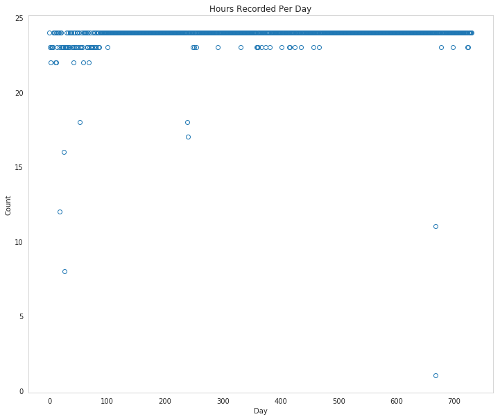
Well, that's odd. It looks like the span is complete, why are there missing hours?

figure, axe = pyplot.subplots(figsize=FIGURE_SIZE)
counts = rides.groupby(["dteday"]).hr.count()
axe.set_title("Hours Recorded Per Day")
axe.set_xlabel("Day")
axe.set_ylabel("Count")
ax = axe.plot(range(len(counts.index)), counts.values, "o", markerfacecolor='None')
date_hours.png

So it looks like some days they didn't manage to record all the hours.

Assuming this is the UC Irvine dataset, this is the description of the variables.

Variable Description
instant record index
dteday date
season season (1:spring, 2:summer, 3:fall, 4:winter)
yr year (0: 2011, 1:2012)
mnth month (1 to 12)
hr hour (0 to 23)
holiday whether day is holiday or not (extracted from Washington D.C. holiday information)
weekday day of the week (0 to 6)
workingday if day is neither weekend nor holiday is 1, otherwise is 0.
weathersit Weather (1, 2, 3, or 4) (see next table)
temp Normalized temperature in Celsius. The values are derived via (t-t_min)/(t_max-t_min), t_min=-8, t_max=+39 (only in hourly scale)
atemp Normalized feeling temperature in Celsius. The values are derived via (t-t_min)/(t_max-t_min), t_min=-16, t_max=+50 (only in hourly scale)
hum Normalized humidity. The values are divided to 100 (max)
windspeed Normalized wind speed. The values are divided to 67 (max)
casual count of casual users
registered count of registered users
cnt count of total rental bikes including both casual and registered

weathersit

Value Meaning
1 Clear, Few clouds, Partly cloudy, Partly cloudy
2 Mist + Cloudy, Mist + Broken clouds, Mist + Few clouds, Mist
3 Light Snow, Light Rain + Thunderstorm + Scattered clouds, Light Rain + Scattered clouds
4 Heavy Rain + Ice Pallets + Thunderstorm + Mist, Snow + Fog

Checking out the data

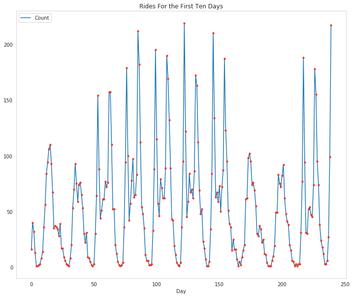
This dataset has the number of riders for each hour of each day from January 1, 2011 to December 31, 2012. The number of riders is split between casual and registered and summed up in the cnt column. You can see the first few rows of the data above.

Below is a plot showing the number of bike riders over the first 10 days or so in the data set (some days don't have exactly 24 entries in the data set, so it's not exactly 10 days). You can see the hourly rentals here. This data is pretty complicated! The weekends have lower over all ridership and there are spikes when people are biking to and from work during the week. Looking at the data above, we also have information about temperature, humidity, and windspeed, all of these likely affecting the number of riders. You'll be trying to capture all this with your model.

figure, axe = pyplot.subplots(figsize=FIGURE_SIZE)
axe.set_title("Rides For the First Ten Days")
first_ten = rides[:24*10]
plot_lines = axe.plot(range(len(first_ten)), first_ten.cnt, label="Count")
lines = axe.plot(range(len(first_ten)), first_ten.cnt,
                 '.',
                 markeredgecolor="r")
axe.set_xlabel("Day")
legend = axe.legend(plot_lines, ["Count"], loc="upper left")
riders_first_ten_days.png

Dummy variables

Here we have some categorical variables like season, weather, month. To include these in our model, we'll need to make binary dummy variables. This is simple to do with Pandas thanks to get_dummies.

dummy_fields = ['season', 'weathersit', 'mnth', 'hr', 'weekday']
for each in dummy_fields:
    dummies = pandas.get_dummies(rides[each], prefix=each, drop_first=False)
    rides = pandas.concat([rides, dummies], axis=1)

fields_to_drop = ['instant', 'dteday', 'season', 'weathersit', 
                  'weekday', 'atemp', 'mnth', 'workingday', 'hr']
data = rides.drop(fields_to_drop, axis=1)
print(data.head())
   yr  holiday  temp   hum  windspeed  casual  registered  cnt  season_1  \
0   0        0  0.24  0.81        0.0       3          13   16         1   
1   0        0  0.22  0.80        0.0       8          32   40         1   
2   0        0  0.22  0.80        0.0       5          27   32         1   
3   0        0  0.24  0.75        0.0       3          10   13         1   
4   0        0  0.24  0.75        0.0       0           1    1         1   

   season_2    ...      hr_21  hr_22  hr_23  weekday_0  weekday_1  weekday_2  \
0         0    ...          0      0      0          0          0          0   
1         0    ...          0      0      0          0          0          0   
2         0    ...          0      0      0          0          0          0   
3         0    ...          0      0      0          0          0          0   
4         0    ...          0      0      0          0          0          0   

   weekday_3  weekday_4  weekday_5  weekday_6  
0          0          0          0          1  
1          0          0          0          1  
2          0          0          0          1  
3          0          0          0          1  
4          0          0          0          1  

[5 rows x 59 columns]

Scaling target variables

To make training the network easier, we'll standardize each of the continuous variables. That is, we'll shift and scale the variables such that they have zero mean and a standard deviation of 1.

The scaling factors are saved so we can go backwards when we use the network for predictions.

quant_features = ['casual', 'registered', 'cnt', 'temp', 'hum', 'windspeed']
# Store scalings in a dictionary so we can convert back later
scaled_features = {}
for each in quant_features:
    mean, std = data[each].mean(), data[each].std()
    scaled_features[each] = [mean, std]
    data.loc[:, each] = (data[each] - mean)/std

Splitting the data into training, testing, and validation sets

We'll save the data for the last approximately 21 days to use as a test set after we've trained the network. We'll use this set to make predictions and compare them with the actual number of riders.

Save data for approximately the last 21 days.

LAST_TWENTY_ONE = -21 * 24 
test_data = data[LAST_TWENTY_ONE:]

Now remove the test data from the data set .

data = data[:LAST_TWENTY_ONE]

Separate the data into features and targets.

target_fields = ['cnt', 'casual', 'registered']
features, targets = data.drop(target_fields, axis=1), data[target_fields]
test_features, test_targets = (test_data.drop(target_fields, axis=1),
                               test_data[target_fields])

We'll split the data into two sets, one for training and one for validating as the network is being trained. Since this is time series data, we'll train on historical data, then try to predict on future data (the validation set).

Hold out the last 60 days or so of the remaining data as a validation set

LAST_SIXTY = -60 * 24
train_features, train_targets = features[:LAST_SIXTY], targets[:LAST_SIXTY]
val_features, val_targets = features[LAST_SIXTY:], targets[LAST_SIXTY:]

Time to build the network

Below you'll build your network. We've built out the structure. You'll implement both the forward pass and backwards pass through the network. You'll also set the hyperparameters: the learning rate, the number of hidden units, and the number of training passes.

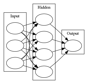
graph = Digraph(comment="Neural Network", format="png")
graph.attr(rankdir="LR")

with graph.subgraph(name="cluster_input") as cluster:
    cluster.attr(label="Input")
    cluster.node("a", "")
    cluster.node("b", "")
    cluster.node("c", "")

with graph.subgraph(name="cluster_hidden") as cluster:
    cluster.attr(label="Hidden")
    cluster.node("d", "")
    cluster.node("e", "")
    cluster.node("f", "")
    cluster.node("g", "")

with graph.subgraph(name="cluster_output") as cluster:
    cluster.attr(label="Output")
    cluster.node("h", "")


graph.edges(["ad", "ae", "af", "ag",
             "bd", "be", "bf", "bg",
             "cd", "ce", "cf", "cg"])

graph.edges(["dh", 'eh', "fh", "gh"])

graph.render("graphs/network.dot")
graph
network.dot.png

The network has two layers, a hidden layer and an output layer. The hidden layer will use the sigmoid function for activations. The output layer has only one node and is used for the regression, the output of the node is the same as the input of the node. That is, the activation function is \(f(x)=x\). A function that takes the input signal and generates an output signal, but takes into account the threshold, is called an activation function. We work through each layer of our network calculating the outputs for each neuron. All of the outputs from one layer become inputs to the neurons on the next layer. This process is called forward propagation.

We use the weights to propagate signals forward from the input to the output layers in a neural network. We use the weights to also propagate error backwards from the output back into the network to update our weights. This is called backpropagation.

Hint: You'll need the derivative of the output activation function (\(f(x) = x\)) for the backpropagation implementation. If you aren't familiar with calculus, this function is equivalent to the equation \(y = x\). What is the slope of that equation? That is the derivative of \(f(x)\).

Below, you have these tasks:

  1. Implement the sigmoid function to use as the activation function. Set `self.activation_function` in `__init__` to your sigmoid function.
  2. Implement the forward pass in the `train` method.
  3. Implement the backpropagation algorithm in the `train` method, including calculating the output error.
  4. Implement the forward pass in the `run` method.

In the my_answers.py file, fill out the TODO sections as specified

from my_answers import NeuralNetwork

Mean Squared Error

def MSE(y, Y):
    return numpy.mean((y-Y)**2)

Unit tests

Run these unit tests to check the correctness of your network implementation. This will help you be sure your network was implemented correctly befor you starting trying to train it. These tests must all be successful to pass the project.

inputs = numpy.array([[0.5, -0.2, 0.1]])
targets = numpy.array([[0.4]])

test_w_i_h = numpy.array([[0.1, -0.2],
                          [0.4, 0.5],
                          [-0.3, 0.2]])
test_w_h_o = numpy.array([[0.3],
                          [-0.1]])

The TestMethods Class

class TestMethods(unittest.TestCase):

    ##########
    # Unit tests for data loading
    ##########

    def test_data_path(self):
        # Test that file path to dataset has been unaltered
        self.assertTrue(data_path.lower() == EXPECTED_DATA_PATH)

    def test_data_loaded(self):
        # Test that data frame loaded
        self.assertTrue(isinstance(rides, pandas.DataFrame))

    ##########
    # Unit tests for network functionality
    ##########

    def test_activation(self):
        network = NeuralNetwork(3, 2, 1, 0.5)
        # Test that the activation function is a sigmoid
        self.assertTrue(numpy.all(network.activation_function(0.5) == 1/(1+numpy.exp(-0.5))))

    def test_train(self):
        # Test that weights are updated correctly on training
        network = NeuralNetwork(3, 2, 1, 0.5)
        network.weights_input_to_hidden = test_w_i_h.copy()
        network.weights_hidden_to_output = test_w_h_o.copy()

        network.train(inputs, targets)
        expected = numpy.array([[ 0.37275328], 
                                [-0.03172939]])
        actual = network.weights_hidden_to_output
        self.assertTrue(
            numpy.allclose(expected, actual),
            "(weights hidden to output) Expected {} Actual: {}".format(
                expected, actual))
        expected = numpy.array([[ 0.10562014, -0.20185996], 
                                [0.39775194, 0.50074398], 
                                [-0.29887597, 0.19962801]])
        actual = network.weights_input_to_hidden
        self.assertTrue(
            numpy.allclose(actual,
                           expected), #, 0.1),
            "(weights input to hidden) Expected: {} Actual: {}".format(
                expected,
                actual))
        return

    def test_run(self):
        # Test correctness of run method
        network = NeuralNetwork(3, 2, 1, 0.5)
        network.weights_input_to_hidden = test_w_i_h.copy()
        network.weights_hidden_to_output = test_w_h_o.copy()

        self.assertTrue(numpy.allclose(network.run(inputs), 0.09998924))

suite = unittest.TestLoader().loadTestsFromModule(TestMethods())
unittest.TextTestRunner().run(suite)
.....
----------------------------------------------------------------------
Ran 5 tests in 0.006s

OK

Training the network

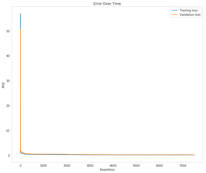
Here you'll set the hyperparameters for the network. The strategy here is to find hyperparameters such that the error on the training set is low, but you're not overfitting to the data. If you train the network too long or have too many hidden nodes, it can become overly specific to the training set and will fail to generalize to the validation set. That is, the loss on the validation set will start increasing as the training set loss drops.

You'll also be using a method know as Stochastic Gradient Descent (SGD) to train the network. The idea is that for each training pass, you grab a random sample of the data instead of using the whole data set. You use many more training passes than with normal gradient descent, but each pass is much faster. This ends up training the network more efficiently. You'll learn more about SGD later.

Choose the number of iterations

This is the number of batches of samples from the training data we'll use to train the network. The more iterations you use, the better the model will fit the data. However, this process can have sharply diminishing returns and can waste computational resources if you use too many iterations. You want to find a number here where the network has a low training loss, and the validation loss is at a minimum. The ideal number of iterations would be a level that stops shortly after the validation loss is no longer decreasing.

Choose the learning rate

This scales the size of weight updates. If this is too big, the weights tend to explode and the network fails to fit the data. Normally a good choice to start at is 0.1; however, if you effectively divide the learning rate by n_records, try starting out with a learning rate of 1. In either case, if the network has problems fitting the data, try reducing the learning rate. Note that the lower the learning rate, the smaller the steps are in the weight updates and the longer it takes for the neural network to converge.

Choose the number of hidden nodes

In a model where all the weights are optimized, the more hidden nodes you have, the more accurate the predictions of the model will be. (A fully optimized model could have weights of zero, after all.) However, the more hidden nodes you have, the harder it will be to optimize the weights of the model, and the more likely it will be that suboptimal weights will lead to overfitting. With overfitting, the model will memorize the training data instead of learning the true pattern, and won't generalize well to unseen data.

Try a few different numbers and see how it affects the performance. You can look at the losses dictionary for a metric of the network performance. If the number of hidden units is too low, then the model won't have enough space to learn and if it is too high there are too many options for the direction that the learning can take. The trick here is to find the right balance in number of hidden units you choose. You'll generally find that the best number of hidden nodes to use ends up being between the number of input and output nodes.

Set the hyperparameters in you myanswers.py file:

from my_answers import iterations, learning_rate, hidden_nodes, output_nodes
N_i = train_features.shape[1]
network = NeuralNetwork(N_i, hidden_nodes, output_nodes, learning_rate)
losses = {'train':[], 'validation':[]}
print("Inputs: {}, Hidden: {}, Output: {}, Learning Rate: {}".format(
    N_i,
    hidden_nodes,
    output_nodes,
    learning_rate))
print("Starting {} repetitions".format(iterations))
for iteration in range(iterations):
    # Go through a random batch of 128 records from the training data set
    batch = numpy.random.choice(train_features.index, size=128)
    X, y = train_features.loc[batch].values, train_targets.loc[batch]['cnt']

    network.train(X, y)

    # Printing out the training progress
    train_loss = MSE(network.run(train_features).T, train_targets['cnt'].values)
    val_loss = MSE(network.run(val_features).T, val_targets['cnt'].values)
    if not iteration % 500:
        sys.stdout.write("\nProgress: {:2.1f}".format(100 * iteration/iterations)
                         + "% ... Training loss: " 
                         + "{:.5f}".format(train_loss)
                         + " ... Validation loss: {:.5f}".format(val_loss))
        sys.stdout.flush()

    losses['train'].append(train_loss)
    losses['validation'].append(val_loss)
Inputs: 56, Hidden: 28, Output: 1, Learning Rate: 0.4
Starting 7500 repetitions

Progress: 0.0% ... Training loss: 1.09774 ... Validation loss: 1.74283
Progress: 6.7% ... Training loss: 0.27687 ... Validation loss: 0.44356
Progress: 13.3% ... Training loss: 0.24134 ... Validation loss: 0.42289
Progress: 20.0% ... Training loss: 0.20681 ... Validation loss: 0.38749
Progress: 26.7% ... Training loss: 0.16536 ... Validation loss: 0.31655
Progress: 33.3% ... Training loss: 0.13105 ... Validation loss: 0.25414
Progress: 40.0% ... Training loss: 0.10072 ... Validation loss: 0.21108
Progress: 46.7% ... Training loss: 0.08929 ... Validation loss: 0.18401
Progress: 53.3% ... Training loss: 0.07844 ... Validation loss: 0.16669
Progress: 60.0% ... Training loss: 0.07380 ... Validation loss: 0.15336
Progress: 66.7% ... Training loss: 0.07580 ... Validation loss: 0.18654
Progress: 73.3% ... Training loss: 0.06308 ... Validation loss: 0.15848
Progress: 80.0% ... Training loss: 0.06632 ... Validation loss: 0.17960
Progress: 86.7% ... Training loss: 0.05954 ... Validation loss: 0.15988
Progress: 93.3% ... Training loss: 0.05809 ... Validation loss: 0.16016
figure, axe = pyplot.subplots(figsize=FIGURE_SIZE)
axe.set_title("Error Over Time")
axe.set_ylabel("MSE")
axe.set_xlabel("Repetition")
axe.plot(range(len(losses["train"])), losses['train'], label='Training loss')
lines = axe.plot(range(len(losses["validation"])), losses['validation'], label='Validation loss')
legend = axe.legend()
losses.png

Check out your predictions

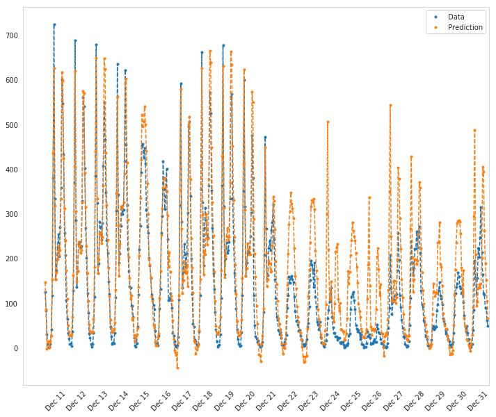
Here, use the test data to view how well your network is modeling the data. If something is completely wrong here, make sure each step in your network is implemented correctly.

fig, axe = pyplot.subplots(figsize=FIGURE_SIZE)

mean, std = scaled_features['cnt']
predictions = network.run(test_features) * std + mean
expected = (test_targets['cnt'] * std + mean).values
axe.plot(expected, '.', label='Data')
axe.plot(expected, linestyle="--", color="tab:blue", label=None)
axe.plot(predictions,linestyle="--", color="tab:orange", label=None)
axe.plot(predictions, ".", label='Prediction')
axe.set_xlim(right=len(predictions))
legend = axe.legend()

dates = pandas.to_datetime(rides.loc[test_data.index]['dteday'])
dates = dates.apply(lambda d: d.strftime('%b %d'))
axe.set_xticks(numpy.arange(len(dates))[12::24])
_ = axe.set_xticklabels(dates[12::24], rotation=45)
count.png

How well does the model predict the data?

It looks like it does better initially and then over-predicts the peaks later on.

Where does it fail?

It doesn't anticipate the drop-off in ridershp as the holidays come around.

Why does it fail where it does?

Although there might be holidays noted (at least for Christmas), it probably isn't reflecting the extreme change in behavior that the holidays bring about in the United States.

More Variations

def train_this(hidden_nodes:int, learning_rate:float,
               output_nodes:int=1, 
               input_nodes: int=N_i,
               repetitions: int=100,
               emit: bool=True):
    """Trains the network using the given values

    Args:
     hidden_nodes: number of nodes in the hidden layer
     learning_rate: amount to change the weights during backpropagation
     output_nodes: number of nodes in the output layer
     input_nodes: number of nodes in the input layer
     repetitions: number of times to train the model
     emit: print information

    Returns:
     test error, losses: MSE against test, dict of losses
    """
    network = NeuralNetwork(input_nodes, hidden_nodes, output_nodes,
                            learning_rate)
    losses = {'train':[], 'validation':[]}
    last_validation_loss = -1
    if emit:        
        print(
            ("Inputs: {}, Hidden: {}, Output: {}, Learning Rate: {}, "
             "Repetitions: {}").format(
                 input_nodes,
                 hidden_nodes,
                 output_nodes,
                 learning_rate, 
                 repetitions))
    reported = False
    for iteration in range(repetitions):
        # Go through a random batch of 128 records from the training data set
        batch = numpy.random.choice(train_features.index, size=128)
        X, y = (train_features.iloc[batch].values,
                train_targets.iloc[batch]['cnt'])
        network.train(X, y)

        train_loss = MSE(network.run(train_features).T, train_targets['cnt'].values)
        val_loss = MSE(network.run(val_features).T, val_targets['cnt'].values)
        losses['train'].append(train_loss)
        losses['validation'].append(val_loss)
        if last_validation_loss == -1:
            last_validation_loss = val_loss[0] 
        if val_loss[0] > last_validation_loss and not reported:
            reported = True
            if emit:
                print("Repetition {} Validation Loss went up by {}".format(
                iteration + 1,
                val_loss[0] - last_validation_loss))
        last_validation_loss = val_loss[0]

    predictions = network.run(test_features)
    expected = (test_targets['cnt']).values
    test_error = MSE(predictions.T, expected)[0]
    if emit:
        print(("Training Error: {:.5f}, "
               "Validation Error: {:.5f}, "
               "Test Error: {:.2f}").format(
                   losses["train"][-1][0],
                   losses["validation"][-1][0],
                   test_error))
    return test_error, losses, network
Parameters = namedtuple(
    "Parameters",
    "hidden_nodes learning_rate trials losses test_error network".split())
def grid_search(hidden_nodes: list, learning_rates: list, trials: list,
                max_train_error = 0.09, max_validation_error=0.18,
                emit_training:bool=False):
    """does a search for the best parameters

    Args:
     hidden_nodes: list of number of hidden nodes
     learning rates: list of how much to update the weights
     trials: list of number of times to train
     max_train_error: upper ceiling for training error
     max_validation_error: upper ceilining for acceptable validation error
     emit_training: print the statements during training
    """
    best = 1000
    if not type(trials) is list:
        trials = [trials]
    for node_count in hidden_nodes:
        for rate in learning_rates:
            for trial in trials:
                test_error, losses, network = train_this(node_count, rate,
                                                         repetitions=trial,
                                                         emit=emit_training)
                if test_error < best:
                    print("New Best: {:.2f} (Hidden: {}, Learning Rate: {:.2f})".format(
                        test_error,
                        node_count,
                        rate))
                    best = test_error
                    best_parameters = Parameters(hidden_nodes=node_count,
                                                 learning_rate=rate,
                                                 trials=trials,
                                                 losses=losses,
                                                 test_error=test_error,
                                                 network=network)
                print()
    return best_parameters
parameters = grid_search(
    hidden_nodes=[14, 28, 42, 56],
    learning_rates=[0.1, 0.01, 0.001],
    trials=200)
New Best: 0.53 (Hidden: 14, Learning Rate: 0.10)


New Best: 0.47 (Hidden: 28, Learning Rate: 0.10)


New Best: 0.44 (Hidden: 42, Learning Rate: 0.10)


New Best: 0.42 (Hidden: 56, Learning Rate: 0.10)


parameters = grid_search([42, 56], [0.1, 0.01, 0.001], trials=300)
New Best: 0.45 (Hidden: 42, Learning Rate: 0.10)


New Best: 0.42 (Hidden: 56, Learning Rate: 0.10)


So, I wouldn't have guessed it, but the 56 node model does best with a reasonably large learning rate.

parameters = grid_search([56, 112], [0.1, 0.2], trials=200)
New Best: 0.44 (Hidden: 56, Learning Rate: 0.10)

New Best: 0.41 (Hidden: 56, Learning Rate: 0.20)


Weird.

parameters = grid_search([56], [0.2, 0.3], trials=300, emit_training=True)
Inputs: 56, Hidden: 56, Output: 1, Learning Rate: 0.2, Repetitions: 300
Repetition 2 Validation Loss went up by 1.2119413344400733
Training Error: 0.42973, Validation Error: 0.71298, Test Error: 0.36
New Best: 0.36 (Hidden: 56, Learning Rate: 0.20)

Inputs: 56, Hidden: 56, Output: 1, Learning Rate: 0.3, Repetitions: 300
Repetition 2 Validation Loss went up by 47.942730166612094
Training Error: 0.69836, Validation Error: 1.20312, Test Error: 0.63

figure, axe = pyplot.subplots(figsize=FIGURE_SIZE)
axe.set_title("Error Over Time")
axe.set_ylabel("MSE")
axe.set_xlabel("Repetition")
losses = parameters.losses
axe.plot(range(len(losses["train"])), losses['train'], label='Training loss')
lines = axe.plot(range(len(losses["validation"])), losses['validation'], label='Validation loss')
legend = axe.legend()
better_losses.png

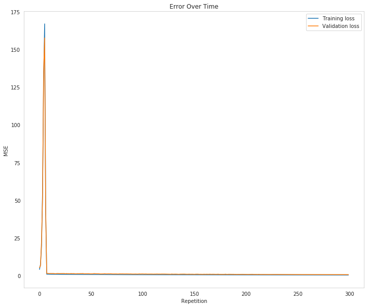
It looks like going over 100 doesn't really help the model a lot, or at all, really.

parameters = grid_search([56], [0.2, 0.3], trials=300, emit_training=True)
Inputs: 56, Hidden: 56, Output: 1, Learning Rate: 0.2, Repetitions: 300
Repetition 2 Validation Loss went up by 0.29155647125413564
Training Error: 0.46915, Validation Error: 0.77756, Test Error: 0.36
New Best: 0.36 (Hidden: 56, Learning Rate: 0.20)

Inputs: 56, Hidden: 56, Output: 1, Learning Rate: 0.3, Repetitions: 300
Repetition 2 Validation Loss went up by 68.10510030432465
Training Error: 0.63604, Validation Error: 1.07500, Test Error: 0.58

start = datetime.now()
parameters = grid_search([56], [0.2], 2000)
print("Elapsed: {}".format(datetime.now() - start))
New Best: 0.27 (Hidden: 56, Learning Rate: 0.20)

Elapsed: 0:02:20.654989
start = datetime.now()
parameters = grid_search([56], [0.2], 1000)
print("Elapsed: {}".format(datetime.now() - start))
New Best: 0.29 (Hidden: 56, Learning Rate: 0.20)

Elapsed: 0:01:51.175404

I just checked the rubric and you need a training loss below 0.09 and a validation loss below 0.18, regardless of the test loss.

start = datetime.now()
parameters = grid_search([28, 42, 56], [0.01, 0.1, 0.2], 100, emit_training=True)
print("Elapsed: {}".format(datetime.now() - start))
Inputs: 56, Hidden: 28, Output: 1, Learning Rate: 0.01, Repetitions: 100
Repetition 10 Validation Loss went up by 0.0005887216742490597
Training Error: 0.92157, Validation Error: 1.36966, Test Error: 0.69
New Best: 0.69 (Hidden: 28, Learning Rate: 0.01)

Inputs: 56, Hidden: 28, Output: 1, Learning Rate: 0.1, Repetitions: 100
Repetition 7 Validation Loss went up by 0.06008857123483735
Training Error: 0.65584, Validation Error: 1.09581, Test Error: 0.52
New Best: 0.52 (Hidden: 28, Learning Rate: 0.10)

Inputs: 56, Hidden: 28, Output: 1, Learning Rate: 0.2, Repetitions: 100
Repetition 4 Validation Loss went up by 0.010135891697978794
Training Error: 0.61391, Validation Error: 0.99344, Test Error: 0.47
New Best: 0.47 (Hidden: 28, Learning Rate: 0.20)

Inputs: 56, Hidden: 42, Output: 1, Learning Rate: 0.01, Repetitions: 100
Repetition 2 Validation Loss went up by 0.0016900520112179684
Training Error: 0.87851, Validation Error: 1.31872, Test Error: 0.66

Inputs: 56, Hidden: 42, Output: 1, Learning Rate: 0.1, Repetitions: 100
Repetition 3 Validation Loss went up by 0.08058311852052547
Training Error: 0.66637, Validation Error: 1.09371, Test Error: 0.53

Inputs: 56, Hidden: 42, Output: 1, Learning Rate: 0.2, Repetitions: 100
Repetition 3 Validation Loss went up by 0.08181869722819135
Training Error: 0.60174, Validation Error: 0.99664, Test Error: 0.47

Inputs: 56, Hidden: 56, Output: 1, Learning Rate: 0.01, Repetitions: 100
Repetition 4 Validation Loss went up by 0.0015646480595301604
Training Error: 0.93732, Validation Error: 1.36061, Test Error: 0.72

Inputs: 56, Hidden: 56, Output: 1, Learning Rate: 0.1, Repetitions: 100
Repetition 2 Validation Loss went up by 0.03097966349747283
Training Error: 0.67087, Validation Error: 1.07306, Test Error: 0.51

Inputs: 56, Hidden: 56, Output: 1, Learning Rate: 0.2, Repetitions: 100
Repetition 2 Validation Loss went up by 9.947099886932289
Training Error: 0.65815, Validation Error: 1.17712, Test Error: 0.52

Elapsed: 0:00:47.842652
start = datetime.now()
parameters = grid_search([28], [0.01, 0.1, 0.2], 1000, emit_training=True)
print("Elapsed: {}".format(datetime.now() - start))
Inputs: 56, Hidden: 28, Output: 1, Learning Rate: 0.01, Repetitions: 1000
Repetition 2 Validation Loss went up by 0.002750823237845479
Training Error: 0.71460, Validation Error: 1.28385, Test Error: 0.59
New Best: 0.59 (Hidden: 28, Learning Rate: 0.01)

Inputs: 56, Hidden: 28, Output: 1, Learning Rate: 0.1, Repetitions: 1000
Repetition 5 Validation Loss went up by 0.09885352252565549
Training Error: 0.31086, Validation Error: 0.48591, Test Error: 0.33
New Best: 0.33 (Hidden: 28, Learning Rate: 0.10)

Inputs: 56, Hidden: 28, Output: 1, Learning Rate: 0.2, Repetitions: 1000
Repetition 2 Validation Loss went up by 0.09560269140958688
Training Error: 0.28902, Validation Error: 0.44905, Test Error: 0.33

Elapsed: 0:01:59.136160
start = datetime.now()
parameters = grid_search([28], [0.1, 0.2], 2000, emit_training=True)
print("Elapsed: {}".format(datetime.now() - start))
Inputs: 56, Hidden: 28, Output: 1, Learning Rate: 0.1, Repetitions: 2000
Repetition 2 Validation Loss went up by 0.06973195973646384
Training Error: 0.28625, Validation Error: 0.45083, Test Error: 0.29
New Best: 0.29 (Hidden: 28, Learning Rate: 0.10)

Inputs: 56, Hidden: 28, Output: 1, Learning Rate: 0.2, Repetitions: 2000
Repetition 3 Validation Loss went up by 0.037295970545350166
Training Error: 0.26864, Validation Error: 0.43831, Test Error: 0.32

Elapsed: 0:02:35.122622
start = datetime.now()
parameters = grid_search([28], [0.05], 4000, emit_training=True)
print("Elapsed: {}".format(datetime.now() - start))
Inputs: 56, Hidden: 28, Output: 1, Learning Rate: 0.1, Repetitions: 4000
Repetition 4 Validation Loss went up by 0.039021584745929205
Training Error: 0.27045, Validation Error: 0.44738, Test Error: 0.29
New Best: 0.29 (Hidden: 28, Learning Rate: 0.10)

Elapsed: 0:02:36.990482
start = datetime.now()
parameters = grid_search([28], [0.2], 5000, emit_training=True)
print("Elapsed: {}".format(datetime.now() - start))
Inputs: 56, Hidden: 28, Output: 1, Learning Rate: 0.2, Repetitions: 5000
Repetition 4 Validation Loss went up by 0.32617394730848104
Training Error: 0.18017, Validation Error: 0.32432, Test Error: 0.24
New Best: 0.24 (Hidden: 28, Learning Rate: 0.20)

Elapsed: 0:03:05.664176
start = datetime.now()
parameters = grid_search([28], [0.2, 0.3], 6000, emit_training=True)
print("Elapsed: {}".format(datetime.now() - start))
Inputs: 56, Hidden: 28, Output: 1, Learning Rate: 0.2, Repetitions: 6000
Repetition 3 Validation Loss went up by 0.18572519005609722
Training Error: 0.22969, Validation Error: 0.38789, Test Error: 0.35
New Best: 0.35 (Hidden: 28, Learning Rate: 0.20)

Inputs: 56, Hidden: 28, Output: 1, Learning Rate: 0.3, Repetitions: 6000
Repetition 3 Validation Loss went up by 1.6850265407570482
Training Error: 0.08168, Validation Error: 0.20003, Test Error: 0.24
New Best: 0.24 (Hidden: 28, Learning Rate: 0.30)

Elapsed: 0:07:30.082137
start = datetime.now()
parameters = grid_search([28], [0.3, 0.4], 7000, emit_training=True)
print("Elapsed: {}".format(datetime.now() - start))
Inputs: 56, Hidden: 28, Output: 1, Learning Rate: 0.3, Repetitions: 7000
Repetition 3 Validation Loss went up by 0.4652683795507646
Training Error: 0.07100, Validation Error: 0.19299, Test Error: 0.29
New Best: 0.29 (Hidden: 28, Learning Rate: 0.30)

Inputs: 56, Hidden: 28, Output: 1, Learning Rate: 0.4, Repetitions: 7000
Repetition 2 Validation Loss went up by 8.612689644792866
Training Error: 0.05771, Validation Error: 0.19188, Test Error: 0.22
New Best: 0.22 (Hidden: 28, Learning Rate: 0.40)

Elapsed: 0:09:06.729922
start = datetime.now()
parameters = grid_search([28], [0.4, 0.5], 7500, emit_training=True)
print("Elapsed: {}".format(datetime.now() - start))
Inputs: 56, Hidden: 28, Output: 1, Learning Rate: 0.4, Repetitions: 7500
Repetition 3 Validation Loss went up by 3.6207932112624386
Training Error: 0.05942, Validation Error: 0.13644, Test Error: 0.16
New Best: 0.16 (Hidden: 28, Learning Rate: 0.40)

Inputs: 56, Hidden: 28, Output: 1, Learning Rate: 0.5, Repetitions: 7500
Repetition 2 Validation Loss went up by 4.101532160572686
Training Error: 0.05710, Validation Error: 0.14214, Test Error: 0.22

Elapsed: 0:09:56.116403
start = datetime.now()
parameters = grid_search([28], [0.4], 8000, emit_training=True)
print("Elapsed: {}".format(datetime.now() - start))
Inputs: 56, Hidden: 28, Output: 1, Learning Rate: 0.4, Repetitions: 8000
Repetition 2 Validation Loss went up by 0.6450181997021212
Training Error: 0.05479, Validation Error: 0.14289, Test Error: 0.24
New Best: 0.24 (Hidden: 28, Learning Rate: 0.40)

Elapsed: 0:05:18.546979

That did worse so it probably overtrains at the 0.4 learning rate. What about 0.3?

start = datetime.now()
parameters = grid_search([28], [0.3], 8000, emit_training=True)
print("Elapsed: {}".format(datetime.now() - start))
Inputs: 56, Hidden: 28, Output: 1, Learning Rate: 0.3, Repetitions: 8000
Repetition 2 Validation Loss went up by 0.3336478297258907
Training Error: 0.06670, Validation Error: 0.16918, Test Error: 0.24
New Best: 0.24 (Hidden: 28, Learning Rate: 0.30)

Elapsed: 0:05:06.761537

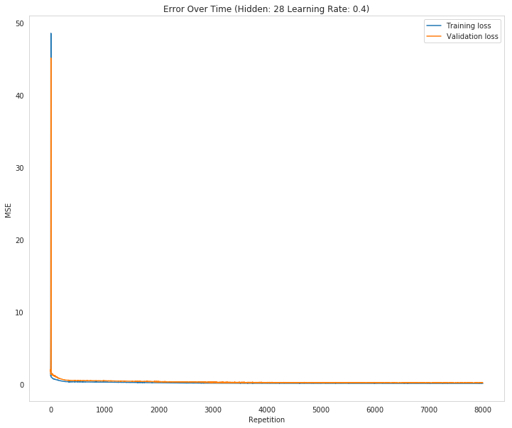
So this did worse than a learning rate of 0.5 at 7500 and much worse than 0.4 at 7500, so maybe that is the optimal (0.4 at 7,500) I'm chasing. It seems king of arbitrary, but it works for the assignment.

The submission is timing out for some reason (it only takes 5 minutes to run but the error says it took more than 7 minutes). I might have to try some compromise runtime.

figure, axe = pyplot.subplots(figsize=FIGURE_SIZE)
axe.set_title("Error Over Time (Hidden: {} Learning Rate: {})".format(parameters.hidden_nodes, parameters.learning_rate))
axe.set_ylabel("MSE")
axe.set_xlabel("Repetition")
losses = parameters.losses
axe.plot(range(len(losses["train"])), losses['train'], label='Training loss')
lines = axe.plot(range(len(losses["validation"])), losses['validation'], label='Validation loss')
legend = axe.legend()
found_losses.png

fig, ax = pyplot.subplots(figsize=FIGURE_SIZE)

mean, std = scaled_features['cnt']
predictions = parameters.network.run(test_features) * std + mean
expected = (test_targets['cnt'] * std + mean).values
ax.plot(expected, '.', label='Data')
ax.plot(predictions.values, ".", label='Prediction')
ax.set_xlim(right=len(predictions))
legend = ax.legend()

dates = pandas.to_datetime(rides.loc[test_data.index]['dteday'])
dates = dates.apply(lambda d: d.strftime('%b %d'))
ax.set_xticks(numpy.arange(len(dates))[12::24])
_ = ax.set_xticklabels(dates[12::24], rotation=45)
best_count.png

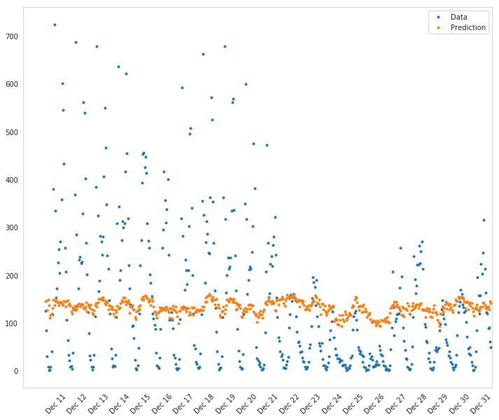
How well does the model predict the data?

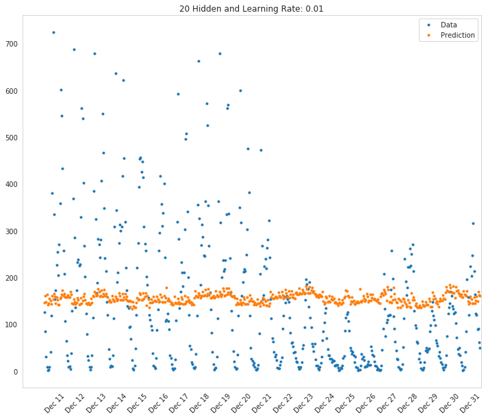
The model seems to not be able to capture all the variations in the data. I don't think it really did well at all.

Where does it fail?

Why does it fail where it does?

better_network = train_this(parameters.hidden_nodes, parameters.learning_rate,
                            repetitions=150, emit=True)
Inputs: 56, Hidden: 19, Output: 1, Learning Rate: 0.01, Repetitions: 150
Repetition 43 Validation Loss went up by 0.0008309723799344582
Training Error: 0.92939, Validation Error: 1.44647, Test Error: 0.62
more_parameters = grid_search([10, 20],
                                [0.1, 0.01],
                                trials=list(range(50, 225, 25)),
                                emit_training=True)
Inputs: 56, Hidden: 10, Output: 1, Learning Rate: 0.1, Repetitions: 50
Repetition 10 Validation Loss went up by 0.013827968028145676
Training Error: 0.92764, Validation Error: 1.45833, Test Error: 0.64
New Best: 0.64 (Hidden: 10, Learning Rate: 0.10)

Inputs: 56, Hidden: 10, Output: 1, Learning Rate: 0.1, Repetitions: 75
Repetition 11 Validation Loss went up by 0.01268617480459655
Training Error: 0.95884, Validation Error: 1.45576, Test Error: 0.67

Inputs: 56, Hidden: 10, Output: 1, Learning Rate: 0.1, Repetitions: 100
Repetition 2 Validation Loss went up by 0.004302293010363778
Training Error: 0.96904, Validation Error: 1.32713, Test Error: 0.74

Inputs: 56, Hidden: 10, Output: 1, Learning Rate: 0.1, Repetitions: 125
Repetition 2 Validation Loss went up by 0.00011567129175471536
Training Error: 0.96480, Validation Error: 1.38193, Test Error: 0.70

Inputs: 56, Hidden: 10, Output: 1, Learning Rate: 0.1, Repetitions: 150
Repetition 2 Validation Loss went up by 0.00525072377638347
Training Error: 0.95649, Validation Error: 1.29823, Test Error: 0.79

Inputs: 56, Hidden: 10, Output: 1, Learning Rate: 0.1, Repetitions: 175
Repetition 6 Validation Loss went up by 0.0184187066638537
Training Error: 0.94033, Validation Error: 1.48648, Test Error: 0.64
New Best: 0.64 (Hidden: 10, Learning Rate: 0.10)

Inputs: 56, Hidden: 10, Output: 1, Learning Rate: 0.1, Repetitions: 200
Repetition 4 Validation Loss went up by 0.006479207709029211
Training Error: 0.96348, Validation Error: 1.38834, Test Error: 0.67

Inputs: 56, Hidden: 10, Output: 1, Learning Rate: 0.01, Repetitions: 50
Repetition 8 Validation Loss went up by 0.00034037805450659597
Training Error: 0.99148, Validation Error: 1.50023, Test Error: 0.71

Inputs: 56, Hidden: 10, Output: 1, Learning Rate: 0.01, Repetitions: 75
Repetition 26 Validation Loss went up by 7.26803968935652e-05
Training Error: 0.94736, Validation Error: 1.42677, Test Error: 0.69

Inputs: 56, Hidden: 10, Output: 1, Learning Rate: 0.01, Repetitions: 100
Repetition 55 Validation Loss went up by 0.0005170583384894734
Training Error: 0.92258, Validation Error: 1.52912, Test Error: 0.64

Inputs: 56, Hidden: 10, Output: 1, Learning Rate: 0.01, Repetitions: 125
Repetition 14 Validation Loss went up by 4.7182200476170166e-05
Training Error: 0.96801, Validation Error: 1.43898, Test Error: 0.69

Inputs: 56, Hidden: 10, Output: 1, Learning Rate: 0.01, Repetitions: 150
Repetition 25 Validation Loss went up by 0.00025169631184263075
Training Error: 0.94769, Validation Error: 1.28473, Test Error: 0.79

Inputs: 56, Hidden: 10, Output: 1, Learning Rate: 0.01, Repetitions: 175
Repetition 2 Validation Loss went up by 0.0011783405140612935
Training Error: 0.95784, Validation Error: 1.38248, Test Error: 0.75

Inputs: 56, Hidden: 10, Output: 1, Learning Rate: 0.01, Repetitions: 200
Repetition 24 Validation Loss went up by 6.126094364189427e-05
Training Error: 0.95839, Validation Error: 1.29311, Test Error: 0.73

Inputs: 56, Hidden: 20, Output: 1, Learning Rate: 0.1, Repetitions: 50
Repetition 4 Validation Loss went up by 0.04115757797958697
Training Error: 0.97326, Validation Error: 1.42168, Test Error: 0.72

Inputs: 56, Hidden: 20, Output: 1, Learning Rate: 0.1, Repetitions: 75
Repetition 3 Validation Loss went up by 0.004544958155855872
Training Error: 0.97079, Validation Error: 1.38326, Test Error: 0.73

Inputs: 56, Hidden: 20, Output: 1, Learning Rate: 0.1, Repetitions: 100
Repetition 2 Validation Loss went up by 0.004455074996461583
Training Error: 0.95492, Validation Error: 1.29813, Test Error: 0.80

Inputs: 56, Hidden: 20, Output: 1, Learning Rate: 0.1, Repetitions: 125
Repetition 3 Validation Loss went up by 0.038516428472006314
Training Error: 0.96063, Validation Error: 1.41134, Test Error: 0.68

Inputs: 56, Hidden: 20, Output: 1, Learning Rate: 0.1, Repetitions: 150
Repetition 4 Validation Loss went up by 0.005238556857821708
Training Error: 0.96022, Validation Error: 1.58371, Test Error: 0.67

Inputs: 56, Hidden: 20, Output: 1, Learning Rate: 0.1, Repetitions: 175
Repetition 4 Validation Loss went up by 0.03291822053421889
Training Error: 0.95138, Validation Error: 1.39820, Test Error: 0.67

Inputs: 56, Hidden: 20, Output: 1, Learning Rate: 0.1, Repetitions: 200
Repetition 2 Validation Loss went up by 0.01721971957045554
Training Error: 0.96676, Validation Error: 1.33802, Test Error: 0.72

Inputs: 56, Hidden: 20, Output: 1, Learning Rate: 0.01, Repetitions: 50
Repetition 2 Validation Loss went up by 0.0016568049054144218
Training Error: 0.90793, Validation Error: 1.36444, Test Error: 0.78

Inputs: 56, Hidden: 20, Output: 1, Learning Rate: 0.01, Repetitions: 75
Repetition 24 Validation Loss went up by 1.0669002188823384e-05
Training Error: 0.93910, Validation Error: 1.43277, Test Error: 0.61
New Best: 0.61 (Hidden: 20, Learning Rate: 0.01)

Inputs: 56, Hidden: 20, Output: 1, Learning Rate: 0.01, Repetitions: 100
Repetition 13 Validation Loss went up by 0.0006819932351833646
Training Error: 0.95953, Validation Error: 1.30219, Test Error: 0.79

Inputs: 56, Hidden: 20, Output: 1, Learning Rate: 0.01, Repetitions: 125
Repetition 2 Validation Loss went up by 0.001983487952677443
Training Error: 0.96503, Validation Error: 1.34180, Test Error: 0.76

Inputs: 56, Hidden: 20, Output: 1, Learning Rate: 0.01, Repetitions: 150
Repetition 2 Validation Loss went up by 0.0014568870668274503
Training Error: 0.95968, Validation Error: 1.34224, Test Error: 0.73

Inputs: 56, Hidden: 20, Output: 1, Learning Rate: 0.01, Repetitions: 175
Repetition 22 Validation Loss went up by 0.0009898893960744726
Training Error: 0.94891, Validation Error: 1.25502, Test Error: 0.81

Inputs: 56, Hidden: 20, Output: 1, Learning Rate: 0.01, Repetitions: 200
Repetition 24 Validation Loss went up by 0.0003693045874550993
Training Error: 0.96222, Validation Error: 1.29511, Test Error: 0.75

best_parameters = grid_search([10, 20, 30, 40], [0.1, 0.01], 100, True)
Inputs: 56, Hidden: 10, Output: 1, Learning Rate: 0.1, Repetitions: 100
Repetition 2 Validation Loss went up by 0.006104362102346439
Training Error: 0.96812, Validation Error: 1.32203, Test Error: 0.76
New Best: 0.76 (Hidden: 10, Learning Rate: 0.10)

Inputs: 56, Hidden: 10, Output: 1, Learning Rate: 0.01, Repetitions: 100
Repetition 16 Validation Loss went up by 0.00020577471034299855
Training Error: 0.96607, Validation Error: 1.30376, Test Error: 0.79

Inputs: 56, Hidden: 20, Output: 1, Learning Rate: 0.1, Repetitions: 100
Repetition 2 Validation Loss went up by 0.018123806353317784
Training Error: 0.95858, Validation Error: 1.28351, Test Error: 0.76
New Best: 0.76 (Hidden: 20, Learning Rate: 0.10)

Inputs: 56, Hidden: 20, Output: 1, Learning Rate: 0.01, Repetitions: 100
Repetition 29 Validation Loss went up by 0.0029168059867459295
Training Error: 0.94895, Validation Error: 1.45710, Test Error: 0.66
New Best: 0.66 (Hidden: 20, Learning Rate: 0.01)

Inputs: 56, Hidden: 30, Output: 1, Learning Rate: 0.1, Repetitions: 100
Repetition 2 Validation Loss went up by 0.045063972993018675
Training Error: 0.96892, Validation Error: 1.50312, Test Error: 0.69

Inputs: 56, Hidden: 30, Output: 1, Learning Rate: 0.01, Repetitions: 100
Repetition 14 Validation Loss went up by 7.233598065781166e-05
Training Error: 0.96606, Validation Error: 1.32913, Test Error: 0.80

Inputs: 56, Hidden: 40, Output: 1, Learning Rate: 0.1, Repetitions: 100
Repetition 3 Validation Loss went up by 0.05076336638491519
Training Error: 0.95920, Validation Error: 1.45843, Test Error: 0.68

Inputs: 56, Hidden: 40, Output: 1, Learning Rate: 0.01, Repetitions: 100
Repetition 7 Validation Loss went up by 0.0006550737027899434
Training Error: 0.97148, Validation Error: 1.36548, Test Error: 0.79

fig, axe = pyplot.subplots(figsize=FIGURE_SIZE)

mean, std = scaled_features['cnt']
predictions = best_parameters.network.run(test_features) * std + mean
expected = (test_targets['cnt'] * std + mean).values
axe.set_title("{} Hidden and Learning Rate: {}".format(best_parameters.hidden_nodes,
                                                       best_parameters.learning_rate))
axe.plot(expected, '.', label='Data')
axe.plot(predictions.values, ".", label='Prediction')
axe.set_xlim(right=len(predictions))
legend = axe.legend()

dates = pandas.to_datetime(rides.loc[test_data.index]['dteday'])
dates = dates.apply(lambda d: d.strftime('%b %d'))
axe.set_xticks(numpy.arange(len(dates))[12::24])
_ = axe.set_xticklabels(dates[12::24], rotation=45)
even_bester_count.png

Student Admissions

Introduction

In this notebook, I'll student admissions to graduate school at UCLA based on three pieces of data:

  • GRE Scores (Test)
  • GPA Scores (Grades)
  • Class rank (1-4)

The dataset originally came from here: http://www.ats.ucla.edu/ (although I couldn't find it).

Imports

From python

from functools import partial

From PyPi

from tabulate import tabulate
import matplotlib.pyplot as pyplot
import numpy
import pandas
import seaborn

This Project

from neurotic.tangles.data_paths import DataPath

Some Set Up

Tables

table = partial(tabulate, showindex=False, tablefmt='orgtbl', headers="keys")

Plotting

%matplotlib inline
seaborn.set(style="whitegrid")
FIGURE_SIZE = (14, 12)

Loading the data

path = DataPath("student_data.csv")
print(path.from_folder)
../../../data/introduction-to-neural-networks/student_data.csv
data = pandas.read_csv(path.from_folder)
print(table(data.head()))
admit gre gpa rank
0 380 3.61 3
1 660 3.67 3
1 800 4 1
1 640 3.19 4
0 520 2.93 4
print(table(data.describe(), showindex=True))
  admit gre gpa rank
count 400 400 400 400
mean 0.3175 587.7 3.3899 2.485
std 0.466087 115.517 0.380567 0.94446
min 0 220 2.26 1
25% 0 520 3.13 2
50% 0 580 3.395 2
75% 1 660 3.67 3
max 1 800 4 4

So we have 400 applicants with about 32% of them being admitted. I don't know how to interpret the rank, maybe that's the quarter the student was in.

Plotting the data

First let's make a plot of our data to see how it looks. In order to have a 2D plot, let's ingore the rank.

Plot Points

def plot_points(data: pandas.DataFrame, identifier: str="All"):
    """Plots the GRE vs GPA

    Args:
     data: frame with the admission, GRE, and GPA data
     identifier: something to identify the data set
    """
    figure, axe = pyplot.subplots(figsize=FIGURE_SIZE)
    axe.set_title("GRE vs GPA and Admissions to UCLA Graduate School ({})".format(identifier))
    X = numpy.array(data[["gre","gpa"]])
    y = numpy.array(data["admit"])
    admitted = X[numpy.argwhere(y==1)]
    rejected = X[numpy.argwhere(y==0)]
    axe.scatter([s[0][0] for s in rejected], [s[0][1] for s in rejected],
                s = 25, color = 'red', edgecolor = 'k', label="Rejected")
    axe.scatter([s[0][0] for s in admitted], [s[0][1] for s in admitted],
                s = 25, color = 'cyan', edgecolor = 'k', label="Admitted")
    axe.set_xlabel('Test (GRE)')
    axe.set_ylabel('Grades (GPA)')
    axe.legend()
    return

GRE Vs GPA

plot_points(data)

gre_vs_gpa.png

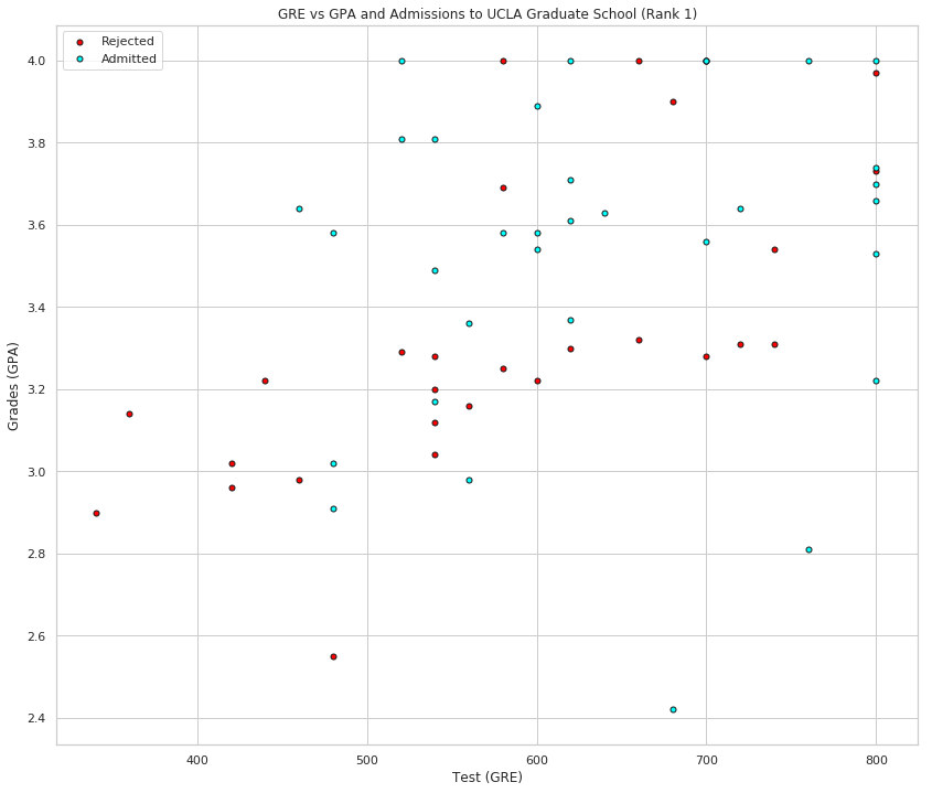
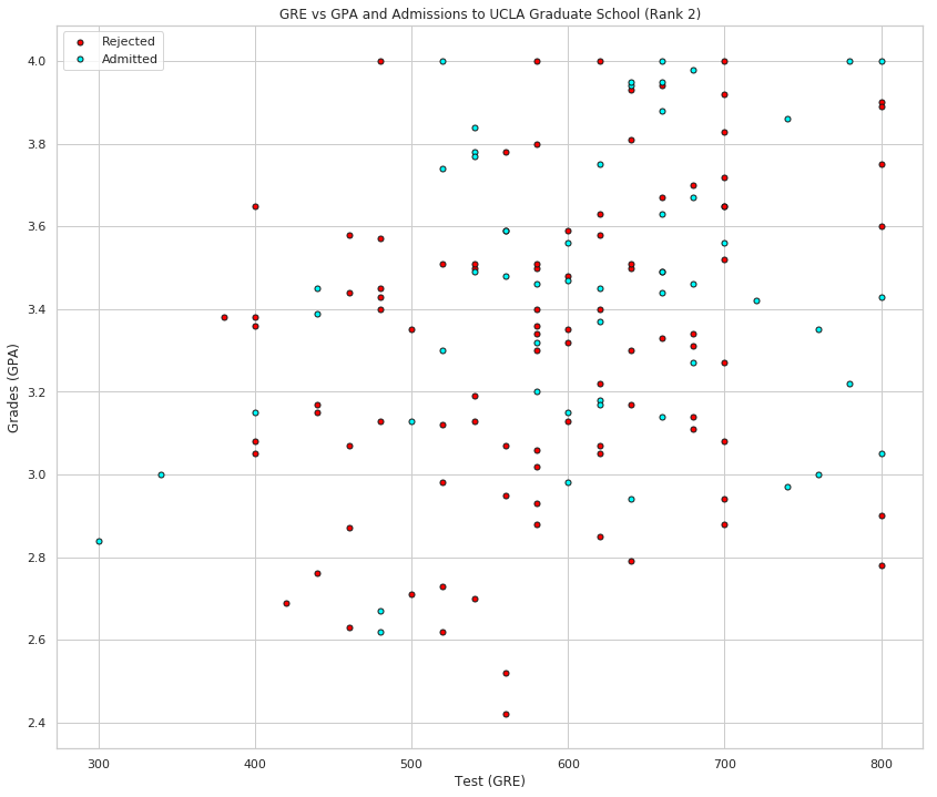
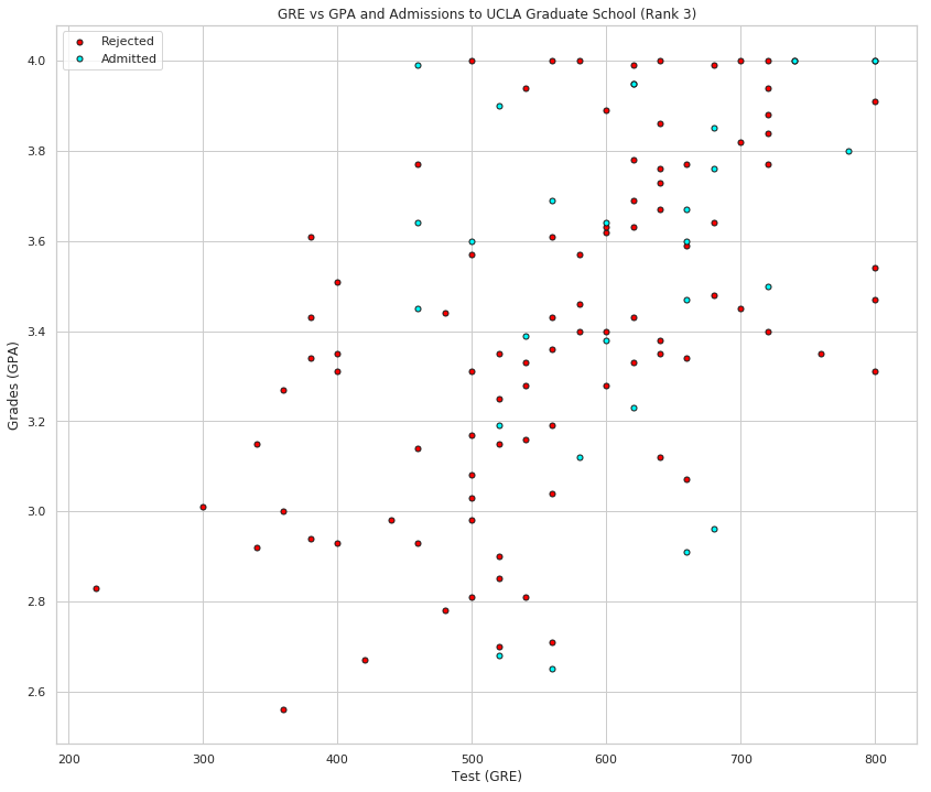
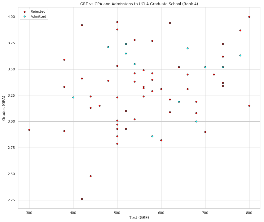
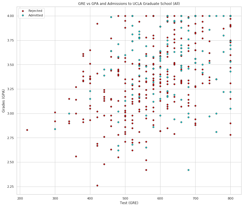
Roughly, it looks like the students with high scores in the grades and test passed, while the ones with low scores didn't, but the data is not as nicely separable as we hoped it would be (to say the least). Maybe it would help to take the rank into account? Let's make 4 plots, each one for each rank.

By Rank

Separating the ranks

data_rank_1 = data[data["rank"]==1]
data_rank_2 = data[data["rank"]==2]
data_rank_3 = data[data["rank"]==3]
data_rank_4 = data[data["rank"]==4]
plot_points(data_rank_1, "Rank 1")

rank_1.png

plot_points(data_rank_2, "Rank 2")

rank_2.png

plot_points(data_rank_3, "Rank 3")

rank_3.png

plot_points(data_rank_4, "Rank 4")

rank_4.png

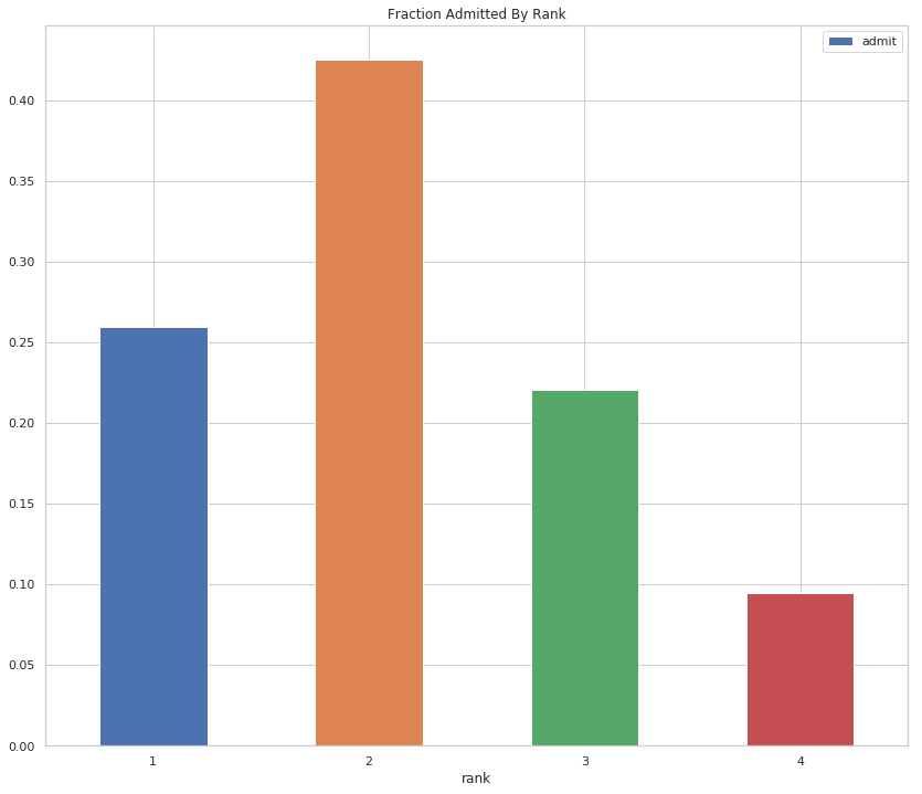
ranked = data.groupby("rank").sum()
fraction = (ranked/data.admit.sum()).reset_index()
print(table(fraction[["rank", "admit"]]))
rank admit
1 0.259843
2 0.425197
3 0.220472
4 0.0944882
figure, axe = pyplot.subplots(figsize=FIGURE_SIZE)
axe.set_title("Fraction Admitted By Rank")
axe = fraction.plot.bar(x="rank", y="admit", ax=axe, rot=False)

rank_bar.png

This looks more promising, as it seems that the lower the rank, the higher the acceptance rate (with rank 2 being the dominant rank among the admitted). Let's use the rank as one of our inputs. In order to do this, we should one-hot encode it.

One-Hot Encoding the Rank

We'll do the one-hot-encoding using pandas' get_dummies function.

one_hot_data = pandas.get_dummies(data, columns=["rank"])
print(table(one_hot_data.head()))
admit gre gpa rank_1 rank_2 rank_3 rank_4
0 380 3.61 0 0 1 0
1 660 3.67 0 0 1 0
1 800 4 1 0 0 0
1 640 3.19 0 0 0 1
0 520 2.93 0 0 0 1

Scaling the data

The next step is to scale the data. We notice that the range for grades is 1.0-4.0, whereas the range for test scores is roughly 200-800, which is much larger. This means our data is skewed, and that makes it hard for a neural network to handle. Let's fit our two features into a range of 0-1, by dividing the grades by 4.0, and the test score by 800.

Making a copy of our data

processed_data = one_hot_data[:]

Scale the columns

processed_data["gpa"] = one_hot_data["gpa"]/4
processed_data["gre"] = one_hot_data["gre"]/800
print(table(processed_data.head()))
admit gre gpa rank_1 rank_2 rank_3 rank_4
0 0.475 0.9025 0 0 1 0
1 0.825 0.9175 0 0 1 0
1 1 1 1 0 0 0
1 0.8 0.7975 0 0 0 1
0 0.65 0.7325 0 0 0 1

Splitting the data into Training and Testing

In order to test our algorithm, we'll split the data into a Training and a Testing set by sampling the data's index (using numpy.random.choice) to find the training set and dropping the sample (pandas.DataFrame.drop) from the data to create the test set. The size of the testing set will be 10% of the total data.

training_size = int(len(processed_data) * 0.9)
sample = numpy.random.choice(processed_data.index,
                             size=training_size, replace=False)
train_data, test_data = processed_data.iloc[sample], processed_data.drop(sample)
print("Number of training samples is", len(train_data))
print("Number of testing samples is", len(test_data))
Number of training samples is 360
Number of testing samples is 40
print(table(train_data[:10]))
admit gre gpa rank_1 rank_2 rank_3 rank_4
0 0.85 0.77 0 0 0 1
1 0.7 0.745 1 0 0 0
0 0.775 0.7625 0 1 0 0
0 0.825 0.8975 0 0 1 0
0 0.75 0.85 0 0 1 0
1 0.65 0.975 0 0 1 0
0 0.775 0.8325 0 0 1 0
0 0.875 0.8175 0 1 0 0
0 0.475 0.835 0 0 1 0
0 0.725 0.84 0 1 0 0
print(table(test_data[:10]))
admit gre gpa rank_1 rank_2 rank_3 rank_4
0 0.5 0.77 0 1 0 0
0 0.875 0.77 0 1 0 0
1 0.875 1 1 0 0 0
0 0.65 0.8225 1 0 0 0
0 0.45 0.785 1 0 0 0
1 0.75 0.7875 0 1 0 0
1 0.725 0.865 0 1 0 0
1 0.775 0.795 0 1 0 0
0 0.725 1 0 1 0 0
1 0.55 0.8625 0 1 0 0

Splitting the data into features and targets (labels)

Now, as a final step before the training, we'll split the data into features (X) and targets (y).

features = train_data.drop('admit', axis="columns")
targets = train_data['admit']
features_test = test_data.drop('admit', axis="columns")
targets_test = test_data['admit']
print(table(features[:10]))
gre gpa rank_1 rank_2 rank_3 rank_4
0.85 0.77 0 0 0 1
0.7 0.745 1 0 0 0
0.775 0.7625 0 1 0 0
0.825 0.8975 0 0 1 0
0.75 0.85 0 0 1 0
0.65 0.975 0 0 1 0
0.775 0.8325 0 0 1 0
0.875 0.8175 0 1 0 0
0.475 0.835 0 0 1 0
0.725 0.84 0 1 0 0
print(table(dict(admit=targets[:10])))
admit
0
1
0
0
0
1
0
0
0
0

Training the 2-layer Neural Network

The following function trains the 2-layer neural network. First, we'll write some helper functions.

Helper Functions

def sigmoid(x):
    return 1 / (1 + numpy.exp(-x))

and the derivative of the sigmoid.

def sigmoid_prime(x):
    return sigmoid(x) * (1-sigmoid(x))
def error_formula(y, output):
    return - y * numpy.log(output) - (1 - y) * numpy.log(1-output)

Backpropagate the error

Now it's your turn to shine. Write the error term. Remember that this is given by the equation \[ -(y-\hat{y}) \sigma'(x) \]

def error_term_formula(y, output):
    return (y - output) * output * (1 - output)

Training

epochs = 1000
learn_rate = 0.5

Training function

def train_nn(features, targets, epochs, learnrate):

    # Use to same seed to make debugging easier
    numpy.random.seed(42)

    n_records, n_features = features.shape
    last_loss = None

    # Initialize weights
    weights = numpy.random.normal(scale=1 / n_features**.5, size=n_features)

    for e in range(epochs):
        del_w = numpy.zeros(weights.shape)
        for x, y in zip(features.values, targets):
            # Loop through all records, x is the input, y is the target

            # Activation of the output unit
            #   Notice we multiply the inputs and the weights here 
            #   rather than storing h as a separate variable 
            output = sigmoid(numpy.dot(x, weights))

            # The error, the target minus the network output
            error = error_formula(y, output)

            # The error term
            #   Notice we calulate f'(h) here instead of defining a separate
            #   sigmoid_prime function. This just makes it faster because we
            #   can re-use the result of the sigmoid function stored in
            #   the output variable
            error_term = error_term_formula(y, output)

            # The gradient descent step, the error times the gradient times the inputs
            del_w += error_term * x

        # Update the weights here. The learning rate times the 
        # change in weights, divided by the number of records to average
        weights += learnrate * del_w / n_records

        # Printing out the mean square error on the training set
        if e % (epochs / 10) == 0:
            out = sigmoid(numpy.dot(features, weights))
            loss = numpy.mean((out - targets) ** 2)
            print("Epoch:", e)
            if last_loss and last_loss < loss:
                print("Train loss: ", loss, "  WARNING - Loss Increasing")
            else:
                print("Train loss: ", loss)
            last_loss = loss
            print("=========")
    print("Finished training!")
    return weights
weights = train_nn(features, targets, epochs, learn_rate)
Epoch: 0
Train loss:  0.27247853979302755
=========
Epoch: 100
Train loss:  0.20397593223991445
=========
Epoch: 200
Train loss:  0.2014297690420066
=========
Epoch: 300
Train loss:  0.2003513187214578
=========
Epoch: 400
Train loss:  0.19984320017443669
=========
Epoch: 500
Train loss:  0.19956325048732546
=========
Epoch: 600
Train loss:  0.19938027609704898
=========
Epoch: 700
Train loss:  0.1992416788675009
=========
Epoch: 800
Train loss:  0.19912513146497982
=========
Epoch: 900
Train loss:  0.19902058341953008
=========
Finished training!

Calculating the Accuracy on the Test Data

test_out = sigmoid(numpy.dot(features_test, weights))
predictions = test_out > 0.5
accuracy = numpy.mean(predictions == targets_test)
print("Prediction accuracy: {:.3f}".format(accuracy))
Prediction accuracy: 0.575

Not horrible, considering the test-set, but not great either.

Try More Epochs

weights_2 = train_nn(features, targets, epochs*2, learn_rate)
Epoch: 0
Train loss:  0.27247853979302755
=========
Epoch: 200
Train loss:  0.2014297690420066
=========
Epoch: 400
Train loss:  0.19984320017443669
=========
Epoch: 600
Train loss:  0.19938027609704898
=========
Epoch: 800
Train loss:  0.19912513146497982
=========
Epoch: 1000
Train loss:  0.19892324129363695
=========
Epoch: 1200
Train loss:  0.19874162735565162
=========
Epoch: 1400
Train loss:  0.19857138905455757
=========
Epoch: 1600
Train loss:  0.1984095079666442
=========
Epoch: 1800
Train loss:  0.1982546851201456
=========
Finished training!
test_out = sigmoid(numpy.dot(features_test, weights_2))
predictions = test_out > 0.5
accuracy = numpy.mean(predictions == targets_test)

print("Prediction accuracy: {:.3f}".format(accuracy))
Prediction accuracy: 0.575

It doesn't make a noticeable difference. Maybe this is the best it can do with only these features.

Gradient Descent Practice

This will implement the basic functions of the Gradient Descent algorithm to find the boundary in a small dataset.

Imports

From Pypi

import matplotlib.pyplot as pyplot
import numpy
import pandas
import seaborn

This Project

from neurotic.tangles.data_paths import DataPath

Helpers

For Plotting

Plot Points

This first function is used to plot the data points as a scatter plot.

def plot_points(X, y, axe=None):
    """Makes a scatter plot

    Args:
     X: array of inputs
     y: array of labels (1's and 0's)
     axe: matplotlib axis object

    Return:
     axe: matplotlib axis
    """
    admitted = X[numpy.argwhere(y==1)]
    rejected = X[numpy.argwhere(y==0)]
    if axe is None:
        figure, axe = pyplot.subplots(figsize=FIGURE_SIZE)
    axe.set_xlim((0, 1))
    axe.set_ylim((0, 1))
    axe.scatter([s[0][0] for s in rejected],
                [s[0][1] for s in rejected],
                s=25, color="blue", edgecolor="k",
                label="Rejects")
    axe.scatter([s[0][0] for s in admitted],
                   [s[0][1] for s in admitted],
                   s=25, color='red', edgecolor='k', label="Accepted")
    axe.legend()
    return axe

Display

The somewhat obscurely named display function is used to plot the separation lines of our model.

def display(m, b, color='g--', axe=None):
    """Makes a line plot

    Args:
     m: slope for the line
     b: intercept for the line
     color: color and line type for plot
     axe: matplotlib axis

    Return:
     axe: matplotlib axis
    """
    if axe is None:
        figure, axe = pyplot.subplots(figsize=FIGURE_SIZE)
    x = numpy.arange(-10, 10, 0.1)
    axe.plot(x, m*x+b, color)
    return axe
%matplotlib inline
seaborn.set(style="whitegrid")
FIGURE_SIZE = (14, 12)

The Data

We'll load the data from data.csv which has three columns - the first two are the inputs and the third is the label that we are trying to predict for the inputs.

path = DataPath("data.csv")

My setup is a little different than the Udacity setup so I'm going to have to get into the habit of setting the file before submission.

print(path.from_folder)
DATA_FILE = path.from_folder
../../../data/introduction_to_neural_networks/data.csv

I'm not sure exactly why, but the data is loaded as a pandas DataFrame (with read_csv) and then converted into two arrays.

data = pandas.read_csv(DATA_FILE, header=None)
X_train = numpy.array(data[[0,1]])
y_train = numpy.array(data[2])
Data Rows Columns
X 100 2
y 100 N/A

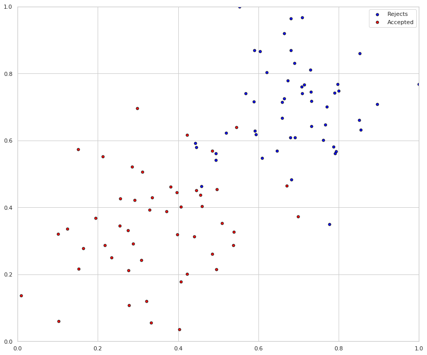
Here's what our data looks like. I don't know what the inputs represent so I didn't label the axes, but it is a plot of the first input variable vs the second input variable, with the colors determined by the labels (y-values).

axe = plot_points(X_train,y_train)

data_scatter.png

The Basic Functions

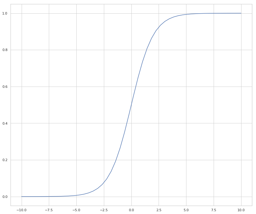
The Sigmoid activation function

This is the function that pushes the probabilities that are produced to be close to 1 or 0 so we can classify the inputs.

\[\sigma(x) = \frac{1}{1+e^{-x}}\]

def sigmoid(x: numpy.ndarray) -> numpy.ndarray:
    """Calculates the sigmoid of x

    Args:
     x: input to classify

    Returns:
     sigmoid of x
    """
    return 1/(1 + numpy.exp(-x))
figure, axe = pyplot.subplots(figsize=FIGURE_SIZE)
x = numpy.linspace(-10, 10)
y = sigmoid(x)
lines = axe.plot(x, y)

sigmoid.png

Output (prediction) formula

This function takes the dot product of the weights and inputs and adds the bias before returning the sigmoid of the calculation.

\[\hat{y} = \sigma(w_1 x_1 + w_2 x_2 + b)\]

def output_formula(features: numpy.ndarray,
                   weights: numpy.ndarray,
                   bias: numpy.ndarray) -> numpy.ndarray:
    """Predicts the outcomes for the inputs

    Args:
     features: inputs variables
     weights: array of weights for the variables
     bias: array of constants to adjust the output

    Returns:
     an array of predicted labels for the inputs
    """
    return sigmoid(features.dot(weights.T) + bias)

Error function (log-loss)

This is used for reporting, since the actual updating of the weights uses the gradient.

\[Error(y, \hat{y}) = - y \log(\hat{y}) - (1-y) \log(1-\hat{y})\]

def error_formula(y: numpy.ndarray, output: numpy.ndarray) -> numpy.ndarray:
    """Calculates the amount of error

    Args:
     y: the true labels
     output: the predicted labels

    Returns:
     amount of error in the output
    """
    return -y * numpy.log(output) - (1 - y) * numpy.log(1 - output)

The function that updates the weights (the gradient descent step)

This makes a prediction of the labels based on the inputs (using output_formula) and then updates the weights and bias based on the amount of error it had in the predictions.

\[ w_i \longrightarrow w_i + \alpha (y - \hat{y}) x_i\\ b \longrightarrow b + \alpha (y - \hat{y})\\ \]

Where \(\alpha\) is our learning rate and \(\hat{y}\) is our prediction for y.

def update_weights(x, y, weights, bias, learning_rate) -> tuple:
    """Updates the weights based on the amount of error

    Args:
     x: inputs
     y: actual labels
     weights: amount to weight each input
     bias: constant to adjust the output
     learning_rate: how much to adjust the weights

    Return:
     w, b: the updated weights
    """
    y_hat = output_formula(x, weights, bias)
    weights +=  learning_rate * (y - y_hat) * x
    bias += learning_rate * (y - y_hat)
    return weights, bias

Training function

This function will help us iterate the gradient descent algorithm through all the data, for a number of epochs. It will also plot the data, and some of the boundary lines obtained as we run the algorithm.

numpy.random.seed(44)
epochs = 100
learning_rate = 0.01
def train(features, targets, epochs, learning_rate, graph_lines=False) -> tuple:
    """Trains a model using gradient descent

    Args:
     features: matrix of inputs
     targets: array of labels for the inputs
     epochs: number of times to train the model
     learning_rate: how much to adjust the weights per epoch

    Returns:
     weights, bias, errors, plot_x, plot_y: What we learned and how we improved
    """
    errors = []
    n_records, n_features = features.shape
    last_loss = None
    weights = numpy.random.normal(scale=1 / n_features**.5, size=n_features)
    bias = 0
    plot_x, plot_y = [], []
    for epoch in range(epochs):
        # train on each row in the training data
        for x, y in zip(features, targets):
            output = output_formula(x, weights, bias)
            error = error_formula(y, output)
            weights, bias = update_weights(x, y, weights, bias, learning_rate)

        # Printing out the log-loss error on the training set
        out = output_formula(features, weights, bias)
        loss = numpy.mean(error_formula(targets, out))
        errors.append(loss)
        if epoch % (epochs / 10) == 0:
            print("\n========== Epoch {} ==========".format(epoch))
            if last_loss and last_loss < loss:
                print("Training loss: ", loss, "  WARNING - Loss Increasing")
            else:
                print("Training loss: ", loss)
            last_loss = loss
            predictions = out > 0.5
            accuracy = numpy.mean(predictions == targets)
            print("Accuracy: ", accuracy)
        if graph_lines and epoch % (epochs / 100) == 0:
            plot_x.append(-weights[0]/weights[1])
            plot_y.append(-bias/weights[1])
    return weights, bias, errors, plot_x, plot_y

Time to train the algorithm.

When we run the function, we'll obtain the following:

  • 10 updates with the current training loss and accuracy
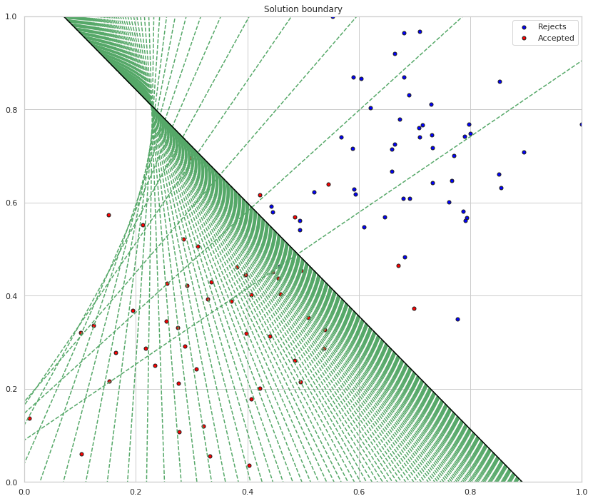
  • A plot of the data and some of the boundary lines obtained. The final one is in black. Notice how the lines get closer and closer to the best fit, as we go through more epochs.
  • A plot of the error function. Notice how it decreases as we go through more epochs.
weights, bias, errors, plot_x, plot_y = train(X_train, y_train, epochs, learning_rate, True)

========== Epoch 0 ==========
Training loss:  0.7135845195381634
Accuracy:  0.4

========== Epoch 10 ==========
Training loss:  0.6225835210454962
Accuracy:  0.59

========== Epoch 20 ==========
Training loss:  0.5548744083669508
Accuracy:  0.74

========== Epoch 30 ==========
Training loss:  0.501606141872473
Accuracy:  0.84

========== Epoch 40 ==========
Training loss:  0.4593334641861401
Accuracy:  0.86

========== Epoch 50 ==========
Training loss:  0.42525543433469976
Accuracy:  0.93

========== Epoch 60 ==========
Training loss:  0.3973461571671399
Accuracy:  0.93

========== Epoch 70 ==========
Training loss:  0.3741469765239074
Accuracy:  0.93

========== Epoch 80 ==========
Training loss:  0.35459973368161973
Accuracy:  0.94

========== Epoch 90 ==========
Training loss:  0.3379273658879921
Accuracy:  0.94

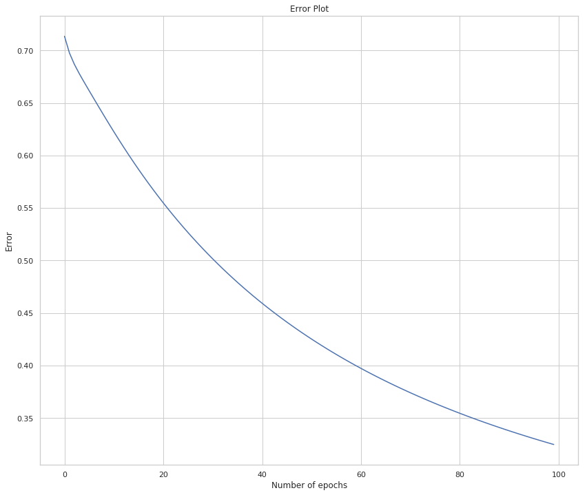
As you can see from the output the accuracy is getting better while the training loss (the mean of the error) is going down.

# Plotting the solution boundary
figure, axe = pyplot.subplots(figsize=FIGURE_SIZE)
axe.set_title("Solution boundary")
learning = zip(plot_x, plot_y)
for learn_x, learn_y in learning:
    display(learn_x, learn_y, axe=axe)
axe = display(-weights[0]/weights[1], -bias/weights[1], 'black', axe)

# Plotting the data
axe = plot_points(X_train, y_train, axe)

training.png

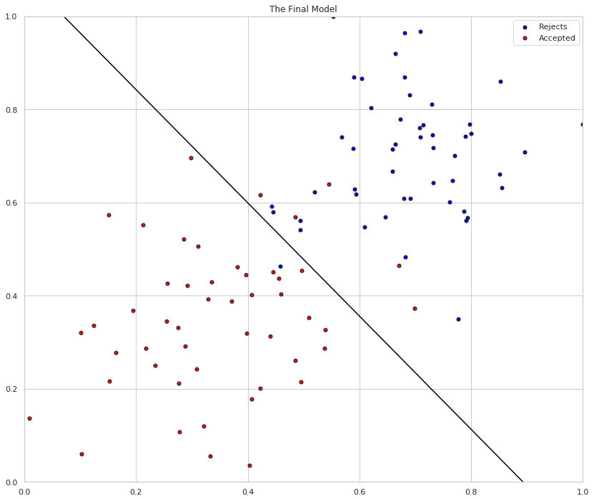
The green lines are the boundary as the model is trained, the black line is the final separator. While pretty, the green lines kind of obscure how well the sepration did. Here's just the final line with the input data.

# Plotting the solution boundary
figure, axe = pyplot.subplots(figsize=FIGURE_SIZE)
axe.set_title("The Final Model")
axe = display(-weights[0]/weights[1], -bias/weights[1], 'black', axe)

# Plotting the data
axe = plot_points(X_train, y_train, axe)

model.png

Finally, this is the amount of error as the model is trained.

# Plotting the error
figure, axe = pyplot.subplots(figsize=FIGURE_SIZE)
axe.set_title("Error Plot")
axe.set_xlabel('Number of epochs')
axe.set_ylabel('Error')
axe = axe.plot(errors)

error.png

Simpler Training

If you squint at the train function you might notice that a considerable amount of it is used for reporting, making it a little harder to read than necessary. This is the same function without the extra reporting.

def only_train(features, targets, epochs, learning_rate) -> tuple:
    """Trains a model using gradient descent

    Args:
     features: matrix of inputs
     targets: array of labels for the inputs
     epochs: number of times to train the model
     learning_rate: how much to adjust the weights per epoch

    Returns:
     weights, bias: Our final model
    """
    number_of_records, number_of_features = features.shape
    weights = numpy.random.normal(scale=1/number_of_records**.5,
                                  size=number_of_features)
    bias = 0
    for epoch in range(epochs):
        for x, y in zip(features, targets):
            weights, bias = update_weights(x, y, weights, bias, learning_rate)
    return weights, bias
weights, bias = only_train(X_train, y_train, epochs, learning_rate)
# Plotting the solution boundary
figure, axe = pyplot.subplots(figsize=FIGURE_SIZE)
axe.set_title("The Final Model")
axe = display(-weights[0]/weights[1], -bias/weights[1], 'black', axe)

# Plotting the data
axe = plot_points(X_train, y_train, axe)

model_2.png

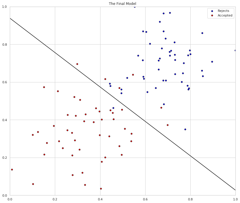
And the model for our linear classifier:

print(("\\[\nw_0 x_0 + w_1 x_1 + b "
       "= {:.2f}x_0 + {:.2f}x_1 + {:.2f}\n\\]").format(weights[0],
                                                       weights[1],
                                                       bias))

\[ w_0 x_0 + w_1 x_1 + b = -3.13x_0 + -3.62x_1 + 3.31 \]

Gradient Descent

What is this about?

We have an initial network and we make a prediction using the inputs. USing the output we can calculate the error. Now that we have the error we need to update our weights - how do we do this? With Gradient Descent, a method that tries to pursue a downward trajectory using the slope of our errors.

How does Gradient Descent Work?

We start by making an initial prediction.

\[ \hat{y} = \sigma(Wx+b) \]

which it turns out is not accurate. We then subtract the gradient of the error (a partial derivative \(\frac{\delta E}{\delta W}\)) multiplied by some learning rate \(\alpha\) that governs how much we are willing to change at each step down the hill.

\[ w'_i \gets w_i - \alpha \frac{\delta E}{\delta W_i}\\ b' \gets b -\alpha \frac{\delta E}{\delta b}\\ \hat{y'} = \sigma(W'x t b') \]

Okay, but what again?

To find our gradient we need to take some derivatives. Let's start with the derivative of our sigmoid.

\[ \sigma' = \sigma(x) (1 - \sigma(x)) \] The lecturer shows the derivation, but take my word for it, this is what it is.

Our error is:

\[ E = -y \ln(\hat{y}) - (1 - y)\ln(1 - \hat{y}) \]

and the derivative of this error:

\[ \frac{\delta}{\delta_{wj}}\hat{y} = \hat{y}(1 - \hat{y}) \dot x_j \]

Trust me, this is the derivation. And the derivation of our error becomes:

\[ \frac{\delta}{\delta w_j} = -(y - \hat{y})x_j \]

and for the bias term we get:

\[ \frac{\delta}{\delta b} = -(y - \hat{y}) \]

And our overall gradient can be written as:

\[ \Delta E = -(y - \hat{y})(x_1, \ldots, x_n, 1) \]

So our gradient is the coordinates of the points times the error. This means that the closer our prediction is to the true value, the smaller the gradient will be, and vice-versa, much like the Perceptron Trick we learned earlier.

So, how do you put it all together?

Okay, this is how you update your weights. First, scale \(\alpha\) to match your data set (divide by the number of rows). \[ \alpha = \frac{1}{m}\alpha \]

Now calculate your new weights.

\[ w_i' \gets w_i + \alpha(y - \hat{y})x_i \]

And the new bias.

\[ b' \gets b \alpha(y - \hat{y}) \]

Compare and Learn

i#t+BEGIN_COMMENT .. title: Compare and Learn .. slug: compare-and-learn .. date: 2018-10-26 10:54:02 UTC-07:00 .. tags: grokking,gradient descent .. category: Grokking .. link: .. description: Introduction to Gradient Descent. .. type: text #+END_COMMENT

Imports

From PyPi

from graphviz import Digraph
import matplotlib.pyplot as pyplot
import numpy
import pandas
import seaborn

Setup the plotting

%matplotlib inline
%config InlineBackend.figure_format='retina'
seaborn.set(style="whitegrid")
FIGURE_SIZE = (14, 12)

What is this about?

The three main steps in training a model are:

  1. Predict
  2. Compare
  3. Learn

Forward Propagation was about the Predict step - we fed some inputs to a network and it output its predictions. Now we're going to look an steps 2 and 3 - Compare and Learn, the steps where we figure out how to improve the weights in our network.

What's the next step after Predict?

As noted above, step 2 is Compare meaning compare our predictions with what we know to be the real answers (so this is supervised learning) and see how well (or bad) we did.

Okay, but then what?

After Compare we move on to the Learn step where we adjust the weights based on the errors we found in Compare. In this case we'll use Gradient Descent to find new weights for the network.

So, how do we find the error again?

There are many different ways to measure error, each with different positive and negative attributes, but in this case we're going to use Mean Squared Error. Here's an example with one measurement.

weight = 0.5
input_value = 0.5
expected = 0.8
actual = weight * input_value
# you implicitly divide by 1 to get the mean of the square
actual_error = (expected - actual)**2
expected_error = 0.3
assert abs(expected_error - actual_error) < 0.01
print("Error: {:.2f}".format(actual_error))
Error: 0.30

Two things to note about the consequences of squaring the error - one is that it's always positive which is useful because you might have both positive and negative errors which would tend to cancel each other out when you take the mean (the actual_error above is a mean with an implied count of 1), even though both positive and negative errors are wrong, the other consequence is that the greater the error, the larger it grows (it follows a parabola instead of a line).

figure, axe = pyplot.subplots(figsize=FIGURE_SIZE)
errors = numpy.linspace(-10, 10)
outputs = numpy.square(errors)
axe.set_xlim((-10, 10))
axe.set_ylim((-10, 100))
axe.set_title("Squared vs Unsquared Errors")
axe.plot(errors, outputs, label="Squared Errors" )
axe.plot(errors, errors, label="Errors")
legend = axe.legend()

squared_error.png

So how do we learn?

One method is Hot-and-Cold Learning. With this method you move your weights a little and pick the one that improves the error-rate. This first example will go back to the one feature network that tries to predict if a team will win using the average number of toes they have.

graph = Digraph(comment="Toes", format="png")
graph.attr(rankdir="LR")
# input layer
graph.node("a", "Toes")

# output layer
graph.node("b", "Win")

# edge
graph.edge("a", "b", label="Weight")
graph.render("graphs/toes_model.dot")
graph

toes_model.dot.png

def toes_model(toes: int, weight: float=0.1) -> float:
    """Predicts if the team will win based on the number of toes

    Return:
     predction: probability of winning
    """
    return toes * weight
def print_error(predicted: float, actual: int, label: str="Toes Model",
                separator: str="\n") -> float:
    """Prints the (mean) squared error

    Args:

     predicted: what the model predicted
     actual: whether the team won or not
     label: something to identify the model
     separator: How to separate the output
    Returns:
     mse: the error
    """
    error = (actual - predicted)**2
    print(separator.join([label,
                          "Predicted: {:.2f}".format(predicted),
                          "Actual: {}".format(actual),
                          "MSE: {:.4f}".format(error)]))
    return error
toes = 8.5
actual = 1
predicted = toes_model(toes)
error_original = print_error(predicted, actual)
Toes Model
Predicted: 0.85
Actual: 1
MSE: 0.0225

So our model has a Mean Squared Error of around 0.02, how do we make it better with the Hot and Cold Method? By trying a larger and smaller weight and using the one that makes the error smaller.

weight_change = 0.01
weight = 0.1
knob_turned_up = toes_model(toes, weight + weight_change)
knob_turned_down = toes_model(toes, weight - weight_change)

error_up = print_error(knob_turned_up, actual, "Turned Up")
print()
error_down = print_error(knob_turned_down, actual, "Turned Down")
Turned Up
Predicted: 0.94
Actual: 1
MSE: 0.0042

Turned Down
Predicted: 0.77
Actual: 1
MSE: 0.0552

Looking at the error, it looks like making the weight higher improved the score, so we should adjust our weight upwards.

if error_original > error_up or error_original > error_down:
    change_direction = -1 if error_down < error_original else 1
    weight_updated = weight + change_direction * weight_change
    prediction = toes_model(toes, weight_updated)
    error_update = print_error(prediction, actual, "Updated Model")
    assert error_update < error_original
else:
    print("Model didn't improve.")
Updated Model
Predicted: 0.94
Actual: 1
MSE: 0.0042

So, this is what machine learning is really about, finding the parameters that give the best prediction. This is why it is often called a search problem - each of your parameters can have a variety of weights (infinite, actually) so what you are doing when you train your model is searching the space of weights to find the set that gives the best outcome for your metric. In this case we are looking to minimize our Mean Squared Error.

Training the Model

Rather than than trying to do the checks one at a time, we can run the Hot and Cold Learning in a loop to tune our model.

weight = 0.5
input_value = 0.5
actual = 0.8
weight_change = 0.001

prediction = toes_model(input_value, weight)
print_error(prediction, actual, "Step    1 Weight: {}".format(weight), "\t")
errors = []
weights = []
optimal_step = False
tolerance = 0.1**8
for step in range(1, 2001):
    prediction = toes_model(input_value, weight)
    error = (print_error(prediction, actual,
                         "Step {:4} Weight: {:.2f}".format(step, weight), "\t")
             if not step % 100 else (prediction - actual)**2)
    errors.append(error)
    if not optimal_step and error < tolerance:
        optimal_step = step - 1
    up_prediction = toes_model(input_value, weight + weight_change)
    down_prediction = toes_model(input_value, weight - weight_change)
    up_error = (up_prediction - actual)**2
    down_error = (down_prediction - actual)**2
    direction = -1 if down_error < up_error else 1
    weight += direction * weight_change
    weights.append(weight)

print("Optimum Reached at Step {}".format(optimal_step))
Step    1 Weight: 0.5   Predicted: 0.25 Actual: 0.8     MSE: 0.3025
Step  100 Weight: 0.60  Predicted: 0.30 Actual: 0.8     MSE: 0.2505
Step  200 Weight: 0.70  Predicted: 0.35 Actual: 0.8     MSE: 0.2030
Step  300 Weight: 0.80  Predicted: 0.40 Actual: 0.8     MSE: 0.1604
Step  400 Weight: 0.90  Predicted: 0.45 Actual: 0.8     MSE: 0.1229
Step  500 Weight: 1.00  Predicted: 0.50 Actual: 0.8     MSE: 0.0903
Step  600 Weight: 1.10  Predicted: 0.55 Actual: 0.8     MSE: 0.0628
Step  700 Weight: 1.20  Predicted: 0.60 Actual: 0.8     MSE: 0.0402
Step  800 Weight: 1.30  Predicted: 0.65 Actual: 0.8     MSE: 0.0227
Step  900 Weight: 1.40  Predicted: 0.70 Actual: 0.8     MSE: 0.0101
Step 1000 Weight: 1.50  Predicted: 0.75 Actual: 0.8     MSE: 0.0026
Step 1100 Weight: 1.60  Predicted: 0.80 Actual: 0.8     MSE: 0.0000
Step 1200 Weight: 1.60  Predicted: 0.80 Actual: 0.8     MSE: 0.0000
Step 1300 Weight: 1.60  Predicted: 0.80 Actual: 0.8     MSE: 0.0000
Step 1400 Weight: 1.60  Predicted: 0.80 Actual: 0.8     MSE: 0.0000
Step 1500 Weight: 1.60  Predicted: 0.80 Actual: 0.8     MSE: 0.0000
Step 1600 Weight: 1.60  Predicted: 0.80 Actual: 0.8     MSE: 0.0000
Step 1700 Weight: 1.60  Predicted: 0.80 Actual: 0.8     MSE: 0.0000
Step 1800 Weight: 1.60  Predicted: 0.80 Actual: 0.8     MSE: 0.0000
Step 1900 Weight: 1.60  Predicted: 0.80 Actual: 0.8     MSE: 0.0000
Step 2000 Weight: 1.60  Predicted: 0.80 Actual: 0.8     MSE: 0.0000
Optimum Reached at Step 1100
figure, axe = pyplot.subplots(figsize=FIGURE_SIZE)
axe.set_title("Hot and Cold Mean Squared Error")
axe.set_xlabel("Training Repetition")
axe.set_ylabel("MSE")
lines = axe.plot(range(len(errors)), errors)

hot_and_cold_error.png

Looking at the output you can see that it reached an error of (nearly) zero at the 1,100th repetition. Based on the plot it looks like it kind of slowed down at the end, which is odd since we're using addition and subtraction, but I guess as the weight gets bigger the proportion of change you add becomes less.

figure, axe = pyplot.subplots(figsize=FIGURE_SIZE)
axe.set_title("Hot and Cold Mean Squared Error vs Weights")
axe.set_xlabel("Weight")
axe.set_ylabel("MSE")
lines = axe.plot(weights, errors, ".")

hot_and_cold_weights_vs_error.png

Our optimal weight appears to be 1.6. Given the simplicity of our model we can check by solving the equation.

\[ prediction = weight \times input\\ weight = \frac{prediction}{input} \]

print(prediction/input_value)
1.6009999999999343

So, that looks about right.

Pros and Cons of Hot and Cold Learning

The main thing that Hot and Cold Learning has going for it is that it is simple to understand and implement. There are a couple of problems with it though:

  • You have to make multiple predictions per knob to make a decision on the change to make.
  • The amount you change the weight at each step can make it impossible to get the right weight, and in most cases you won't have just one input value so it's hard to know what to pick

Is there a better way to update the weights?

With Hot and Cold Learning we make multiple predictions to decide which direction to add a set amount to the weight. But we can instead use the error to change our weight, and in doing so we will change both direction and scale based on the error. In this case error means "pure error", or just the difference between the prediction and the actual value.

\[ error = prediction - actual \]

Since we don't square it the error will be positive if our prediction is too high and negative if it is too low. We don't want to just use the difference, though, because we are adjusting a weight that gets multiplied by the input, so we need to scale the amount of change by the input.

Note that the ordering is now important - you have to subtract the error in the version above and add it if the terms are switched.

\[ adjustment = error * input\\ weights' = weights - adjustment \]

This is the method of Gradient Descent. This is how it looks run on our previous problem.

weight = 0.5
input_value = 0.5
actual = 0.8

prediction = toes_model(input_value, weight)
print_error(prediction, actual, "Step    1 Weight: {}".format(weight), "\t")
errors = []
weights = []
optimal_step = False
tolerance = 0.1**8
optimal_count = 0
print_every = 5
stop_after = 30
for step in range(1, 2001):
    prediction = toes_model(input_value, weight)
    difference = (prediction - actual) * input_value
    weight -= difference
    weights.append(weight)    
    error = (print_error(prediction, actual,
                         "Step {:4} Weight: {:.2f}".format(step, weight), "\t")
             if not step % print_every else (prediction - actual)**2)
    errors.append(error)
    if not optimal_step and error < tolerance:
        optimal_step = step - 1
    if error < tolerance:
        optimal_count += 1
    if optimal_count >= stop_after:
        break
print("Optimum Reached at Step {}".format(optimal_step))
Step    1 Weight: 0.5   Predicted: 0.25 Actual: 0.8     MSE: 0.3025
Step    5 Weight: 1.34  Predicted: 0.63 Actual: 0.8     MSE: 0.0303
Step   10 Weight: 1.54  Predicted: 0.76 Actual: 0.8     MSE: 0.0017
Step   15 Weight: 1.59  Predicted: 0.79 Actual: 0.8     MSE: 0.0001
Step   20 Weight: 1.60  Predicted: 0.80 Actual: 0.8     MSE: 0.0000
Step   25 Weight: 1.60  Predicted: 0.80 Actual: 0.8     MSE: 0.0000
Step   30 Weight: 1.60  Predicted: 0.80 Actual: 0.8     MSE: 0.0000
Step   35 Weight: 1.60  Predicted: 0.80 Actual: 0.8     MSE: 0.0000
Step   40 Weight: 1.60  Predicted: 0.80 Actual: 0.8     MSE: 0.0000
Step   45 Weight: 1.60  Predicted: 0.80 Actual: 0.8     MSE: 0.0000
Step   50 Weight: 1.60  Predicted: 0.80 Actual: 0.8     MSE: 0.0000
Step   55 Weight: 1.60  Predicted: 0.80 Actual: 0.8     MSE: 0.0000
Step   60 Weight: 1.60  Predicted: 0.80 Actual: 0.8     MSE: 0.0000
Optimum Reached at Step 30

So it now hits the optimal solution at the 30th step instead of the 1,100th step (although it really seems to reach it at step 20, I think the difference is a rounding problem).

figure, axe = pyplot.subplots(figsize=FIGURE_SIZE)
axe.set_title("Gradient Descent Mean Squared Error")
axe.set_xlabel("Training Repetition")
axe.set_ylabel("MSE")
lines = axe.plot(range(len(errors)), errors)

gradient_descent_error.png

figure, axe = pyplot.subplots(figsize=FIGURE_SIZE)
axe.set_title("Gradient Descent Mean Squared Error vs Weights")
axe.set_xlabel("Weight")
axe.set_ylabel("MSE")
lines = axe.plot(weights, errors, "o")

gradient_descent_weights_vs_error.png

The plots show what we already saw in the output, that Gradient Descent converges on a solution much faster than Hot and Cold Learning does.

Why multiply the error by the input?

This has three main effects called stopping, negative reversal, and scaling.

What is Stopping?

Stopping refers to the case where the input is 0. If that's the case then we don't want to adjust the weight so multiplying the error by the input nullifies it.

What is Negative Reversal?

The sign of the input changes which direction we want the weight to change, so multiplying it by the input keeps the change moving in the right direction even when the sign of the input changes.

What is Scaling?

The larger the input, the greater the amount of change it will add. This can be a bad thing, since the inputs can now have an outsized (negative) effect.

A Discursion On Derivatives

What we're doing when we train our model to minimize our error. In the Mean Squared Error equation:

\[ MSE = \frac{1}{n} \sum_{i=1}^n ((input \times weight) - actual)^2 \]

The only thing we can change is the weight, the input and actual output is set by the data. So what we're interested in is how the error changes as we change the weight. The relationship between how the output changes in relationship to how the input changes is the derivative. One way to think of the derivative is the slope at a point on a line. If you have a straight line the slope will be the same everywhere on it, but if it is curved then different points will have different slopes.

In our case our input is the weight and the output is the error. If you think about slope as \[\frac{rise}{run}\] you'll notice that the bigger the rise, the bigger the slope (since we're taking it at a point the run is infinitesimal), and it's positive going up and negative going down, so if you think of the plot of the MSE earlier, the further you go away from the center (where the error is zero), the steeper the slope, and moving away from the center is always moving up, so the slope is always positive, and moving toward the center where the error is zero is always moving down, so the slope is negative.

What we want, then, is to move our weights in the opposite direction of the slope. There's more math involved to explain this than I can handle right now, but when we calculate our weight adjustment, we are calculating the derivative, and since we want to move in the opposite direction of the derivative, we negate it. And the further away we are from the true value (where our error is zero), the greater the difference is, as we would expect from the slope of our line.

\[ \Delta = prediction - actual\\ \Delta_{weighted} = \Delta \times input\\ weight' = weight - \Delta_{weighted} \]

When does this work?

Well, it's easier to look at when it doesn't work than when it does.

class OneNode:
    """Implements a single-node network

    Args:
     weight: the starting weight for the edge from the input to the output
     input_value: the input to the node
     actual: the actual output we are trying to predict

     training_steps: how many times to train the model
     tolerance: how close to zero we need our error to be
     print_every: how often to print training status
     stop_after: how many times to keep going after the optimal was found
    """
    def __init__(self, weight: float,
                 input_value: float,
                 actual: float,
                 training_steps: int=200,
                 tolerance: float=0.1**8,
                 print_every: int=5, stop_after: int=30) -> None:
        self.original_weight = weight
        self.weight = weight
        self.input_value = input_value
        self.actual = actual
        self.training_steps = training_steps
        self.tolerance = tolerance
        self.print_every = print_every
        self.stop_after = stop_after
        self._errors = None
        self._weights = None
        self._predictions = None
        return

    @property
    def errors(self) -> list:
        """list of MSE values"""
        if self._errors is None:
            self._errors = []
        return self._errors

    @property
    def weights(self) -> list:
        """List of weights built during training"""
        if self._weights is None:
            self._weights = [self.weight]
        return self._weights

    @property
    def predictions(self) -> list:
        """List of predictions made"""
        if self._predictions is None:
            self._predictions = []
        return self._predictions

    @property
    def prediction(self) -> float:
        """The current model's prediction"""
        return self.weight * self.input_value

    def mean_squared_error(self) -> float:
        """The mean squared error for the prediction"""
        try:
            self.predictions.append(self.prediction)
            return (self.prediction - self.actual)**2
        except OverflowError as error:
            print(error)
            print("prediction: {}".format(self.prediction))
            print("actual: {}".format(self.actual))
        return

    def print_error(self,
                    step: int,
                    separator: str="\t",
                    force_print: bool=False,
                    store_error: bool=True) -> float:
        """Prints the (mean) squared error

       Args:
        step: what step this is
        separator: How to separate the output
        force_print: ignore the step count and print anyway
        store_error: whether to add to the errors
       Returns:
        mse: the error
       """
        error = self.mean_squared_error()
        if store_error:
            self.errors.append(error)
        if force_print or not step % self.print_every:
            print("Input: {} Actual Output: {}".format(self.input_value,
                                                       self.actual))
            print(separator.join(["Step: {}".format(step),
                                  "Weight: {}".format(self.weight),
                                  "Predicted: {:.2f}".format(self.prediction),
                                  "MSE: {:.4f}".format(error)]))
        return error

    def adjust_weight(self) -> None:
        """Takes the gradient descent step"""
        scaled_derivative = (self.prediction - self.actual) * self.input_value
        self.weight -= scaled_derivative
        self.weights.append(self.weight)
        return

    def train(self):
        """Trains our model on the values

       """
        self.reset()
        prediction = self.weight * self.input_value
        optimal_step = optimal_count = 0
        error = self.print_error(1,
                                 force_print=True,
                                 store_error=False)
        for step in range(1, self.training_steps + 1):
            error = self.print_error(step)
            if error is None:
                return

            self.adjust_weight()
            if not optimal_step and error < self.tolerance:
                optimal_step = step - 1
            if error < tolerance:
                optimal_count += 1
            if optimal_count >= self.stop_after:
                break
        print("Optimum Reached at Step {}".format(optimal_step))
        return

    def plot_errors_over_time(self, scale="linear") -> None:
        """Plots the error as it is trained

       Args:
        scale: y-axis scale
       """
        figure, axe = pyplot.subplots(figsize=FIGURE_SIZE)
        axe.set_title("Gradient Descent Mean Squared Error")
        axe.set_xlabel("Training Repetition")
        axe.set_ylabel("MSE")
        axe.set_yscale(scale)
        lines = axe.plot(range(len(self.errors)), self.errors)
        return

    def plot_errors_vs_weights(self, style="o") -> None:
        """Plots errors given weights"""
        figure, axe = pyplot.subplots(figsize=FIGURE_SIZE)
        axe.set_title("Gradient Descent Mean Squared Error vs Weights")
        axe.set_xlabel("Weight")
        axe.set_ylabel("MSE")
        lines = axe.plot(self.weights, self.errors, style)
        return

    def plot_weight_distribution(self) -> None:
        """Plots the distribution of the weights"""
        figure, axe = pyplot.subplots(figsize=FIGURE_SIZE)
        axe.set_title("Distribution Of Weights")
        lines = seaborn.distplot(self.weights)
        return


    def reset(self):
        """Resets the properties"""
        self._errors = None
        self._weights = None
        self._predictions = None
        self.weight = self.original_weight
        return

Really Big Inputs

network = OneNode(weight=0.1, input_value=5, actual=0.1, print_every=30)
network.train()
Input: 5 Actual Output: 0.1
Step: 1 Weight: 0.1     Predicted: 0.50 MSE: 0.1600
Input: 5 Actual Output: 0.1
Step: 30        Weight: -8.496029205125367e+38  Predicted: -4248014602562683567255766167412625375232.00 MSE: 18045628063585794511112671022597693816764790617265863683813015097617735965736960.0000
Input: 5 Actual Output: 0.1
Step: 60        Weight: -2.1654753676302967e+80 Predicted: -1082737683815148355196656106977575165473067380893761893846901009426287310965571584.00       MSE: 1172320891953392254658250331342439625964504567088377053437708818301948653571886896236931555371967400274585017142698424782066192956435576184566862647806273773371392.0000
Input: 5 Actual Output: 0.1
Step: 90        Weight: -5.51938258990998e+121  Predicted: -275969129495499010312802960568845701886516344963538842611688052470072992651229004282112996195046030793242534509005731004416.00      MSE: 76158960434503501277477316231095001035615545032300898123025508833954593912013767638712660721529293958181614329406854402338675069139074333788043867020532267345247209268079568592806683870329999393916410491701860464641755145654976460424275531137024.0000
(34, 'Numerical result out of range')
prediction: 1.5336245888098994e+154
actual: 0.1

So, when the input is too big, the prediction explodes.

network.plot_errors_over_time()

too_big_errors.png

It looks at first like there was no error and then all of a sudden it got huge - but if you look at the scale of the y-axis it maxes out at over \(4\times10^{305}\) and then the overflow error causes it to quit. So when the input is too large, the network goes out of control.

network.plot_errors_vs_weights()

too_big_errors_vs_weights.png So now it looks like there aren't really many weights, but if you look at both the X and Y scales you can see that they're really huge, so most of the points are probably centered around 0 (relative to the overall scale) and then all of a sudden they go crazy on the last two points.
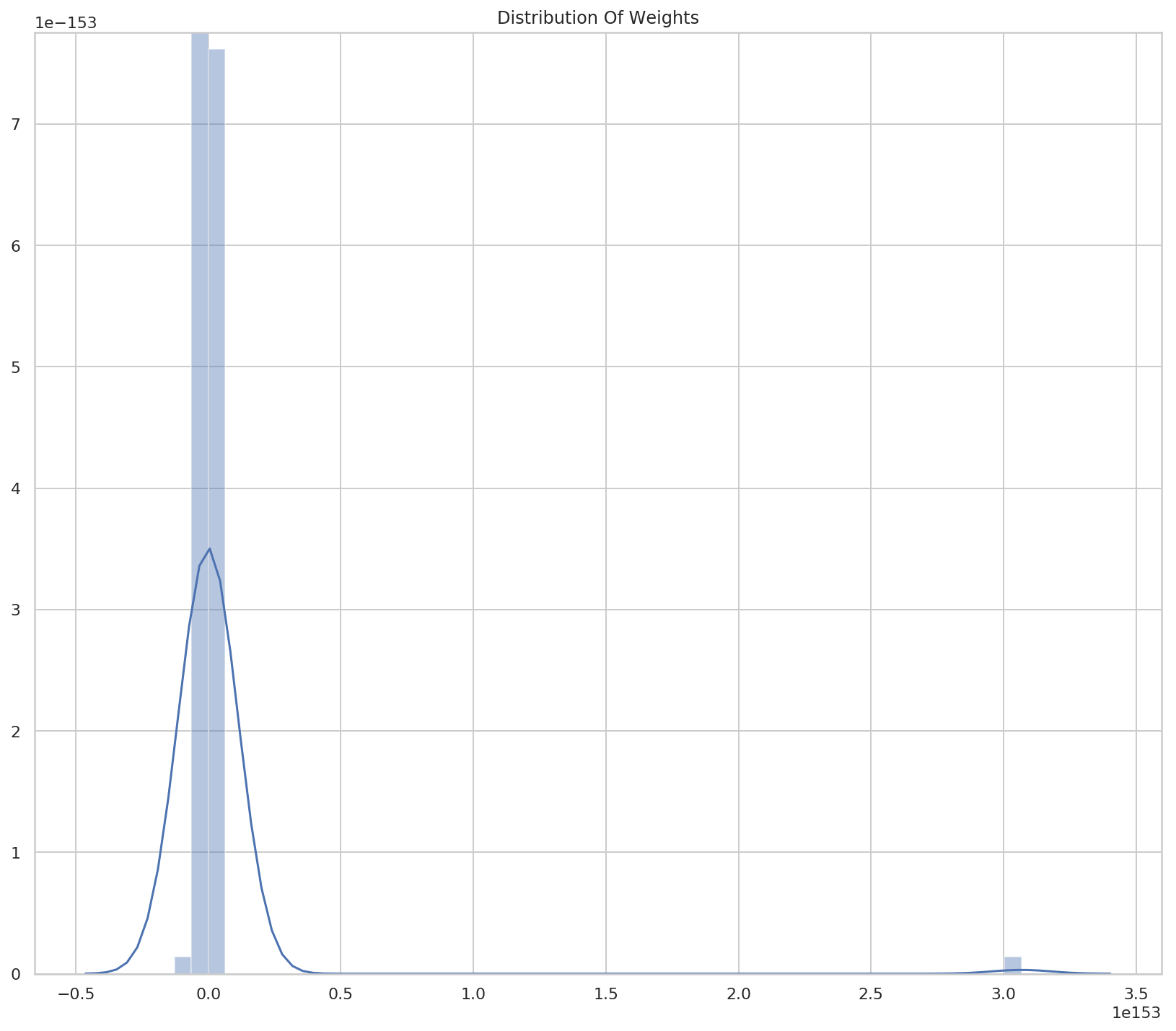
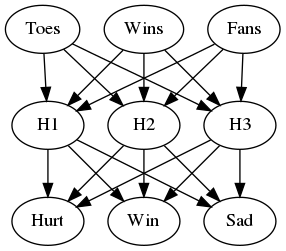
figure, axe
network.plot_weight_distribution()

too_big_distribution_of_weights.png

So we have a small number of weights that are very large. Or a lot of very large weights with a small number of very-very-large weights.

weights = pandas.Series(network.weights)
print(weights.describe())
count     1.130000e+02
mean     2.605805e+151
std      2.888965e+152
min     -1.278020e+152
25%      -6.526920e+74
50%      -1.900000e+00
75%       1.566461e+76
max      3.067249e+153
dtype: float64

So the median is -1.9 and the mean is \(0.6 \times 10^{151}\). Looks like there are some outliers.

Fixing the Big Input Problem

The problem with big inputs is that they cause the gradient descent to explode. Remember our error function:

\[ error = input \times (predicted - actual)\\ = input \times ((input \times weights) - actual) \]

If the input is big the error will be big, and since our correction to the weights is based on the error:

\[ weights' = weights - error \]

our weights can start to swing wildly back and forth with the error growing larger and larger and swinginig between positive and negative numbers. The larger the input, the larger the error, the larger the derivative will be in the opposite direction.

The fix is to only update using a fraction of the correction. We find some value (\(\alpha\)) and multiply it by the change to reduce the influence any one change has. How do we find \(\alpha\)? Well, that turns out to be done by trial and error. If your error goes up as you train, then you probably have to make it smaller.

class AlphaNode(OneNode):
    """Incorporates weight update reduction

    Args:
     alpha: amount to weight the update

     weight: the starting weight for the edge from the input to the output
     input_value: the input to the node
     actual: the actual output we are trying to predict

     training_steps: how many times to train the model
     tolerance: how close to zero we need our error to be
     print_every: how often to print training status
     stop_after: how many times to keep going after the optimal was found
    """
    def __init__(self, alpha: float, *args, **kwargs) -> None:
        self.alpha = alpha
        __class__
        super().__init__(*args, **kwargs)
        return

    def adjust_weight(self) -> None:
        """Takes the gradient descent step with alpha weight"""
        scaled_derivative = (self.prediction - self.actual) * self.input_value
        self.weight -= self.alpha * scaled_derivative
        self.weights.append(self.weight)
        return

Why does this help? Our problem is that the large inputs cause the gradient descent to overshoot past the value that would give zero error and by reducing the amount any one change can have we reduce the likelihood that this will happen.

alpha_network = AlphaNode(alpha=0.1, weight=0.5, input_value=5,
                          actual=0.8, print_every=30)
alpha_network.train()
Input: 5 Actual Output: 0.8
Step: 1 Weight: 0.5     Predicted: 2.50 MSE: 2.8900
Input: 5 Actual Output: 0.8
Step: 30        Weight: -43463.41342612052      Predicted: -217317.07   MSE: 47227055374.1942
Input: 5 Actual Output: 0.8
Step: 60        Weight: -8334186242.344855      Predicted: -41670931211.72      MSE: 1736466508118929965056.0000
Input: 5 Actual Output: 0.8
Step: 90        Weight: -1598089039844441.2     Predicted: -7990445199222206.00 MSE: 63847214481773219178788224499712.0000
Input: 5 Actual Output: 0.8
Step: 120       Weight: -3.064352661386353e+20  Predicted: -1532176330693176459264.00   MSE: 2347564308336405932287023519199639310958592.0000
Input: 5 Actual Output: 0.8
Step: 150       Weight: -5.875928686839428e+25  Predicted: -293796434341971398081118208.00      MSE: 86316344832056315635271476663737243674922770633850880.0000
Input: 5 Actual Output: 0.8
Step: 180       Weight: -1.1267155496783526e+31 Predicted: -56335777483917627928853446918144.00 MSE: 3173719824717480263078840848567916525595895306706307529098395648.0000
Optimum Reached at Step 0

Okay, so that still didn't work, maybe if \(\alpha\) was smaller?

alpha_network.alpha = 0.01
alpha_network.train()
Input: 5 Actual Output: 0.8
Step: 1 Weight: 0.5     Predicted: 2.50 MSE: 2.8900
Input: 5 Actual Output: 0.8
Step: 30        Weight: 0.1600809572142104      Predicted: 0.80 MSE: 0.0000
Input: 5 Actual Output: 0.8
Step: 60        Weight: 0.16000001445750855     Predicted: 0.80 MSE: 0.0000
Optimum Reached at Step 34

So now our model is able to reach the correct value again. Can you figure out what the best \(\alpha\) is ahead of time? The magic eight ball says no. At this point in time the best way to find the hyperparameters for machine learning is to try them until you find the ones that perform the best.

Logistic Regression

What is Logistic Regression?

Logistic Regression is a classification algorithm that estimates the probability of a classification given an input. It is one of the foundations of deep learning.

The Error Function

\[ error = -\frac{1}{m} \sum^m_{i=1} (1-y)\ln(1-\hat{y}) + y \ln \hat{y} \]

To build our model we add weights (W) and a bias term (b) to the error function \(E(W,b)\).

\[ E(W,b) = -\frac{1}{m} \sum^m_{i=1} (1-y_i)\ln(1-\sigma(Wx^{(i)}) + b) + y_i \ln(\sigma(Wx^{(i)} + b)) \]

This is the function for the binary case, but you can generalize it to more cases using this function.

\[ E(W, b) = -\frac{1}{m} \sum^m_{i=1} \sum^n_{j=1} y_{ij} \ln(\hat{y_{ij}}) \]

The goal is to minimize this function to get the best model.

Multi-Class Cross Entropy

Our Probabilities

Weh have three doors behind which could be one of three animals. These are the probabilities that if you open a door, you will find a particular animal behind it.

Animal Door 1 Door 2 Door 3
Duck \(P_{11}\) \(P_{12}\) \(P_{13}\)
Beaver \(P_{21}\) \(P_{22}\) \(P_{23}\)
Walrus \(P_{31}\) \(P_{32}\) \(P_{33}\)

\[ \textit{Cross Entropy} = - \sum^n_{i=1} \sum^m_{j=1} y_{ij} \ln (p_{ij}) \]

So, what does this mean?

Cross Entropy is inversely proportional to the the total probability of an outcome - so the higher the cross entropy you calculate, the less likely it is that the outcome you are looking at will happen.

Okay, but what about this deep-learning stuff?

Imports

From Python

from typing import List

From Pypi

from graphviz import Digraph
import numpy

Typing

This is to develop some type hinting.

Vector = List[float]
Matrix = List[Vector]

What is this about?

I previously looked at a model with multiple inputs and outputs to predict whether a team would win or lose and how the fans would feel in response to the outcome. Now I'm going to stack the network on top of another one to 'deepen' the network.

graph = Digraph(comment="Hidden Layers", format="png")
# input layer
graph.node("A", "Toes")
graph.node("B", "Wins")
graph.node("C", "Fans")

# Hidden Layer
graph.node("D", "H1")
graph.node("E", "H2")
graph.node("F", "H3")

# Output Layer
graph.node("G", "Hurt")
graph.node("H", "Win")
graph.node("I", "Sad")

# Input to hidden edges
graph.edges(["AD", "AE", "AF",
             "BD", "BE", "BF",
             "CD", "CE", "CF",
])

# Hidden to output egdes
graph.edges(["DG", "DH", "DI",
             "EG", "EH", "EI",
             "FG", "FH", "FI",
])
graph.render("graphs/hidden_layer.dot")
graph

hidden_layer.dot.png

These networks between the input and output layers are called hidden layers.

Okay, so how do you implement that?

It works like our previous model except that you insert an extra vector-matrix-multiplication call between the inputs and outputs. For this example I'm going to do it as a class so that I can check the hidden layer's values more easily, but otherwise you would do it using matrices and vectors.

class HiddenLayer:
    """Implements a neural network with one hidden layer

    Args:
     inputs: vector of input values
     input_to_hidden_weights: vector of weights for the first layer
     hidden_to_output_weights: vector of weights of the second layer
    """
    def __init__(self, inputs: Vector, input_to_hidden_weights: Vector,
                 hidden_to_output_weights: Vector) -> None:
        self.inputs = inputs
        self.input_to_hidden_weights = input_to_hidden_weights
        self.hidden_to_output_weights = hidden_to_output_weights
        self._hidden_output = None
        self._predictions = None
        return

    @property
    def hidden_output(self) -> Vector:
        """the output of the hidden layer"""
        if self._hidden_output is None:
            self._hidden_output = self.vector_matrix_multiplication(
                self.inputs,
                self.input_to_hidden_weights)
        return self._hidden_output

    @property
    def predictions(self) -> Vector:
        """Predictions for the inputs"""
        if self._predictions is None:
            self._predictions = self.vector_matrix_multiplication(
                self.hidden_output,
                self.hidden_to_output_weights,
            )
        return self._predictions

    def vector_matrix_multiplication(self, vector: Vector,
                                     matrix: Matrix) -> Vector:
        """calculates the dot-product for each row of the matrix

       Args:
        vector: input with one cell for each row in the matrix
        matrix: input with rows of the same length as the vector

       Returns:
        vector: dot-products for the vector and matrix rows
       """
        vector_length = len(vector)
        assert vector_length == len(matrix)
        rows = range(len(matrix))
        return [self.dot_product(vector, matrix[row]) for row in rows]

    def dot_product(self, vector_1:Vector, vector_2:Vector) -> float:
        """Calculate the dot-product of the two vectors

       Returns:
        dot-product: the dot product of the two vectors
       """
        vector_length = len(vector_1)
        assert vector_length == len(vector_2)
        entries = range(vector_length)
        return sum((vector_1[entry] * vector_2[entry] for entry in entries))

Let's try it out

The Input Layer To Hidden Layer Weights

Toes Wins Fans  
0.1 0.2 -0.1 h0
-0.1 0.1 0.9 h1
0.1 0.4 0.1 h2
input_to_hidden_weights = [[0.1, 0.2, -0.1],
                           [-0.1, 0.1, 0.9],
                           [0.1, 0.4, 0.1]]

The Weights From the Hidden Layer to the Outputs

h0 h1 h2  
0.3 1.1 -0.3 hurt
0.1 0.2 0.0 won
0.0 1.3 0.1 sad
hidden_layer_to_output_weights = [[0.3, 1.1, -0.3],
                                  [0.1, 0.2, 0.0],
                                  [0.0, 1.3, 0.1]]

Testing it Out

toes = [8.5, 9.5, 9.9, 9.0]
wins = [0.65, 0.8, 0.8, 0.9]
fans = [1.2, 1.3, 0.5, 1.0]
expected_hiddens = [0.86, 0.295, 1.23]
expected_outputs = [0.214, 0.145, 0.507]
first_input = [toes[0], wins[0], fans[0]]
network = HiddenLayer(first_input,
                       input_to_hidden_weights,
                       hidden_layer_to_output_weights)
hidden_outputs = network.hidden_output
expected_actual = zip(expected_hiddens, hidden_outputs)
tolerance = 0.1**5
labels = "h0 h1 h2".split()
print("|Node | Expected | Actual")
print("|-+-+-|")
for index, (expected, actual) in enumerate(expected_actual):
    print("|{} | {}| {:.2f}".format(labels[index], expected, actual))
    assert abs(expected - actual) < tolerance
Node Expected Actual
h0 0.86 0.86
h1 0.295 0.29
h2 1.23 1.23
outputs = network.predictions
expected_actual = zip(expected_outputs, outputs)
tolerance = 0.1**3
labels = "Hurt Won Sad".split()
print("|Node | Expected | Actual")
print("|-+-+-|")
for index, (expected, actual) in enumerate(expected_actual):
    print("|{} | {}| {:.3f}".format(labels[index], expected, actual))
    assert abs(expected - actual) < tolerance
Node Expected Actual
Hurt 0.214 0.214
Won 0.145 0.145
Sad 0.507 0.506

Okay, but can we do that with numpy?

def one_hidden_layer(inputs: Vector, weights: Matrix) -> numpy.ndarray:
    """Converts arguments to numpy and calculates predictions

    Args:
     inputs: array of inputs
     weights: matrix with two rows of weights

    Returns:
     predictions: predicted values for each output node
    """
    inputs, weights = numpy.array(inputs), numpy.array(weights)
    hidden = inputs.dot(weights[0].T)
    return hidden.dot(weights[1].T)

One thing to watch out for here is that the dot product won't raise an error if you don't transpose the weights, but you will get the wrong values.

weights = [input_to_hidden_weights,
           hidden_layer_to_output_weights]
outputs = one_hidden_layer(first_input, weights)
expected_actual = zip(expected_outputs, outputs)
tolerance = 0.1**3
labels = "Hurt Won Sad".split()
print("|Node | Expected | Actual")
print("|-+-+-|")
for index, (expected, actual) in enumerate(expected_actual):
    print("|{} | {}| {:.3f}".format(labels[index], expected, actual))
    assert abs(expected - actual) < tolerance
Node Expected Actual
Hurt 0.214 0.214
Won 0.145 0.145
Sad 0.507 0.506

Okay, so what was this about again?

This showed that you can stack networks up and have the outputs of one layer feed into the next until you reach the output layer. This is called Forward Propagation. Although I mentioned deep-learning in the title this really isn't an example yet, it's more like a multilayer perceptron, but it's deeper than two-layers, anyway.

Maximum Likelihood

What is this about?

We want a way to train our neural network based on the data we have - how do we do this? One way is to use maximum likelihood where we give weights based on the past occurrences for each score.

Yeah, okay, but how do you do this?

First, remember that our probability for any point being 0 or 1 is based on the sigmoid.

\[ \hat{y} = \sigma(Wx+b) \]

Where \(\hat{y}\) is the probability that a point is non-negative.

So we can take the product of the sigmoid of all the points in our data set and find the probability that any point is a 1. If we were to find a model that maximized this probability, we would have a model that separated our categories - this is the Maximum Likelihood Model.

To be more specific, we calculate \(\hat{y}\) for all of our training set points and multiply them to get the total probability (multiplication is an AND operation - \(p(a) \land p(b) \land p(c) = p(a) \times p(b) \time p(c)\)) then we adjust our moder to maximize this probability.

The Problem With Products

Each of our probablilities is less than 1, so the more of them you have, the smaller their product will become. What we want to do is use addition - which is where the logarithm comes in.

\[ p(a) * p(b) * p(c) = \log(a) + \log p(b) + \log p(4) \]

Cross Entropy

Our logarithms give us the values that we want to maximize, but another way to look at is as "we want to minimize the error". We can do this by using the negatives of the logarithms to find the error and trying to minimize their sums.

\[ \textit{cross entropy} = -\log p(a) - \log p(b) - \log p(4) \]

More generally:

\[ \textit{Cross Entropy} = -\sum_{i=1}^m y_i \ln(p_i) + (1 - y_i)\ln(1-p_i) \]

Where y is vector of 1's and 0's. When y is 0, the left term is 0 and when y is 1 the right term is 0 so it works as sort of a conditional to choose which term to use.

Okay, but how do we implement this?

Write a function that takes as input two lists Y, P, and returns the float corresponding to their cross-entropy.

import numpy
def cross_entropy(Y, P):
    """calculates the cross entropy of two lists

    Args:
     Y: lists of 1s and 0s
     P: lists of probabilities that Y is 1
    Returns:
     cross-entropy: the cross entropy of the two lists
    """
    Y = numpy.array(Y)
    not_Y = 1 - Y    
    P = numpy.array(P)
    not_P = 1 - P
    return -(Y * numpy.log(P) + not_Y * numpy.log(not_P)).sum()
Y=[1,0,1,1] 
P=[0.4, 0.6, 0.1, 0.5]
expected =  4.8283137373
entropy = cross_entropy(Y, P)
print(entropy)
assert abs(entropy - expected) < 0.1**5
4.828313737302301

One-Hot Encoding

Table of Contents

The Problem

We are dealing with categories - Duck, Beaver, and Walrus - but our classifier works with numbers, what do we do?

One Solution

one-hot encoding, in this context, means taking each of our classifications and creating a column for it and putting a 1 in the row if it matches the column and a 0 otherwise.

Sighting Duck Beaver Walrus
0 1 0 0
1 0 1 0
2 1 0 0
3 0 0 1
4 0 1 0