Dog Breed Classification

Introduction

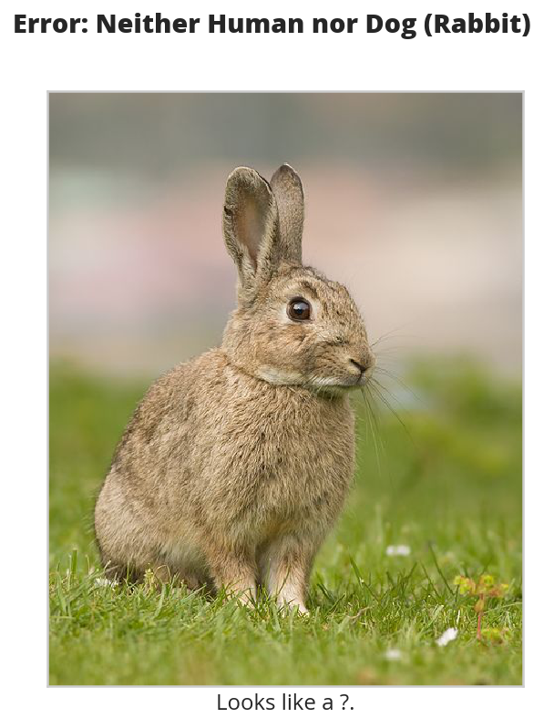
This application is a dog-breed classifier. It takes as input an image and detects if it's an image of either a human or a dog and if it's either one of those then it finds the dog-breed classification that the subject of the image most resembles. If it's neither a human or a dog then it emits an error message. To do this I'm going to try two libraries for each of the human face-detectors and dog detectors and I'm also going to try three Neural Networks to try and classify the dog breeds.

Set Up

This section does some preliminary set-up for the code that comes later.

Imports

Python

from functools import partial
from pathlib import Path
import os
import warnings

From Pypi

from dotenv import load_dotenv
from PIL import Image, ImageFile
from torchvision import datasets
import cv2
import face_recognition
import matplotlib.cbook
warnings.filterwarnings("ignore", category=matplotlib.cbook.mplDeprecation)
import matplotlib.pyplot as pyplot
import matplotlib.image as mpimage
import matplotlib.patches as patches
import numpy
try:
    import pyttsx3
    SPEAKABLE = True
except ImportError:
    print("pyttsx3 not available")
    SPEAKABLE = False
import seaborn
import torch
import torchvision.models as models
import torch.nn as nn
import torch.nn.functional as F
import torch.optim as optimizer
import torchvision.transforms as transforms

This Project

This is code that I wrote to maybe make it easier to work with.

from neurotic.tangles.data_paths import DataPathTwo
from neurotic.tangles.timer import Timer
from neurotic.constants.imagenet_map import imagenet

Plotting

get_ipython().run_line_magic('matplotlib', 'inline')
get_ipython().run_line_magic('config', "InlineBackend.figure_format = 'retina'")
seaborn.set(style="whitegrid",
            rc={"axes.grid": False,
                "font.family": ["sans-serif"],
                "font.sans-serif": ["Open Sans", "Latin Modern Sans", "Lato"],
                "figure.figsize": (8, 6)},
            font_scale=1)

Set the Random Seed

numpy.random.seed(seed=2019)

Check If CUDA Is Available

device = torch.device("cuda" if torch.cuda.is_available() else "cpu")
print(device)
cuda

Handle Truncated Images

There seems to be at least one image that is truncated which will cause an exception when it's loaded so this next setting lets us ignore the error and keep working.

ImageFile.LOAD_TRUNCATED_IMAGES = True

Build the Timer

The timer times how long a code-block takes to run so that if I run it more than once I'll know if it will take a while.

timer = Timer(beep=SPEAKABLE)

The Data Paths

The data-sets are hosted online and need to be downloaded.

I've already downloaded them and put the path to the folders in a .env file so this next block gets the paths so we can load the data later.

The Model Path

The models turn out to take up a lot of space so I'm saving them outside of the repository.

MODEL_PATH = DataPathTwo(folder_key="MODELS")

Dog Paths

This is a class to hold the paths for the dog Images

class DogPaths:
    """holds the paths to the dog images"""
    def __init__(self) -> None:
        self._main = None
        self._training = None
        self._testing = None
        self._validation = None
        self._breed_count = None
        load_dotenv()
        return

    @property
    def main(self) -> DataPathTwo:
        """The path to the main folder"""
        if self._main is None:
            self._main = DataPathTwo(folder_key="DOG_PATH")
        return self._main

    @property
    def training(self) -> DataPathTwo:
        """Path to the training images"""
        if self._training is None:
            self._training = DataPathTwo(folder_key="DOG_TRAIN")
        return self._training

    @property
    def validation(self) -> DataPathTwo:
        """Path to the validation images"""
        if self._validation is None:
            self._validation = DataPathTwo(folder_key="DOG_VALIDATE")
        return self._validation

    @property
    def testing(self) -> DataPathTwo:
        """Path to the testing images"""
        if self._testing is None:
            self._testing = DataPathTwo(folder_key="DOG_TEST")
        return self._testing

    @property
    def breed_count(self) -> int:
        """Counts the number of dog breeds

        This assumes that the training folder has all the breeds
        """
        if self._breed_count is None:
            self._breed_count = len(set(self.training.folder.iterdir()))
        return self._breed_count

    def check(self) -> None:
        """Checks that the folders are valid

        Raises: 
         AssertionError: folder doesn't exist
        """
        self.main.check_folder()
        self.training.check_folder()
        self.validation.check_folder()
        self.testing.check_folder()
        return

Now I'll build the dog-paths.

dog_paths = DogPaths()

Human Path

This is the path to the downloaded Labeled Faces in the Wild data set.

human_path = DataPathTwo(folder_key="HUMAN_PATH")

Check the Paths

This makes sure that the folders exist and shows where they are.

print(dog_paths.main.folder)
print(dog_paths.training.folder)
print(dog_paths.testing.folder)
print(dog_paths.validation.folder)
dog_paths.check()
print(human_path.folder)
human_path.check_folder()
/home/hades/data/datasets/dog-breed-classification/dogImages
/home/hades/data/datasets/dog-breed-classification/dogImages/train
/home/hades/data/datasets/dog-breed-classification/dogImages/test
/home/hades/data/datasets/dog-breed-classification/dogImages/valid
/home/hades/data/datasets/dog-breed-classification/lfw

Count The Breeds

To build the neural network I'll need to know how many dog breeds there are. I made it an attribute of the DogPath class and I'll just inspect it here.

print("Number of Dog Breeds: {}".format(dog_paths.breed_count))
Number of Dog Breeds: 133

Load the Files

For this first part we're going to load in all the files and ignore the train-validation-test split for the dog-images.

timer.start()
human_files = numpy.array(list(human_path.folder.glob("*/*")))
dog_files = numpy.array(list(dog_paths.main.folder.glob("*/*/*")))
timer.end()
Started: 2019-01-13 14:05:09.566221
Ended: 2019-01-13 14:05:42.932863
Elapsed: 0:00:33.366642
print('There are {:,} total human images.'.format(len(human_files)))
print('There are {:,} total dog images.'.format(len(dog_files)))
There are 13,233 total human images.
There are 8,351 total dog images.

So we have a bit more human images than dog images.

Some Helper Code

This is code meant to help with the other code.

Tee

I wrote this for the jupyter notebook because it loses the output if the server disconnects. I think it will also make it easier to use multiproccessing so I can train things in parallel. But I don't think I'm using it right now.

class Tee:
    """Save the input to a file and print it

    Args:
     log_name: name to give the log    
     directory_path: path to the directory for the file
    """
    def __init__(self, log_name: str, 
                 directory_name: str="../../../logs/dog-breed-classifier") -> None:
        self.directory_name = directory_name
        self.log_name = log_name
        self._path = None
        self._log = None
        return

    @property
    def path(self) -> Path:
        """path to the log-file"""
        if self._path is None:
            self._path = Path(self.directory_name).expanduser()
            assert self._path.is_dir()
            self._path = self._path.joinpath(self.log_name)
        return self._path

    @property
    def log(self):
        """File object to write log to"""
        if self._log is None:
            self._log = self.path.open("w", buffering=1)
        return self._log

    def __call__(self, line: str) -> None:
        """Writes to the file and stdout

        Args:
         line: text to emit
        """
        self.log.write("{}\n".format(line))
        print(line)
        return

F1 Scorer

I'm going to be comparing two models for both the humans and dogs, this scorer will focus on the F1 score, but will emit some other information as well.

 class F1Scorer:
     """Calculates the F1 and other scores

     Args:
      predictor: callable that gets passed and image and outputs boolean
      true_images: images that should be predicted as True
      false_images: images that shouldn't be matched by the predictor
      done_message: what to announce when done
     """
     def __init__(self, predictor: callable, true_images:list,
                  false_images: list,
                  done_message: str="Scoring Done") -> None:
         self.predictor = predictor
         self.true_images = true_images
         self.false_images = false_images
         self.done_message = done_message
         self._timer = None
         self._false_image_predictions = None
         self._true_image_predictions = None
         self._false_positives = None
         self._false_negatives = None
         self._true_positives = None
         self._true_negatives = None
         self._false_positive_rate = None
         self._precision = None
         self._recall = None
         self._f1 = None
         self._accuracy = None
         self._specificity = None
         return

     @property
     def timer(self) -> Timer:
         if self._timer is None:
             self._timer = Timer(message=self.done_message, emit=False)
         return self._timer

     @property
     def false_image_predictions(self) -> list:
         """Predictions made on the false-images"""
         if self._false_image_predictions is None:
             self._false_image_predictions = [self.predictor(str(image))
                                              for image in self.false_images]
         return self._false_image_predictions

     @property
     def true_image_predictions(self) -> list:
         """Predictions on the true-images"""
         if self._true_image_predictions is None:
             self._true_image_predictions = [self.predictor(str(image))
                                             for image in self.true_images]
         return self._true_image_predictions

     @property
     def true_positives(self) -> int:
         """count of correct positive predictions"""
         if self._true_positives is None:
             self._true_positives = sum(self.true_image_predictions)
         return self._true_positives

     @property
     def false_positives(self) -> int:
         """Count of incorrect positive predictions"""
         if self._false_positives is None:
             self._false_positives = sum(self.false_image_predictions)
         return self._false_positives

     @property
     def false_negatives(self) -> int:
         """Count of images that were incorrectly classified as negative"""
         if self._false_negatives is None:
             self._false_negatives = len(self.true_images) - self.true_positives
         return self._false_negatives

     @property
     def true_negatives(self) -> int:
         """Count of images that were correctly ignored"""
         if self._true_negatives is None:
             self._true_negatives = len(self.false_images) - self.false_positives
         return self._true_negatives

     @property
     def accuracy(self) -> float:
         """fraction of correct predictions"""
         if self._accuracy is None:
             self._accuracy = (
                 (self.true_positives + self.true_negatives)
                 /(len(self.true_images) + len(self.false_images)))
         return self._accuracy

     @property
     def precision(self) -> float:
         """True-Positive with penalty for false positives"""
         if self._precision is None:
             self._precision = self.true_positives/(
                 self.true_positives + self.false_positives)
         return self._precision

     @property
     def recall(self) -> float:
         """fraction of correct images correctly predicted"""
         if self._recall is None:
             self._recall = (
                 self.true_positives/len(self.true_images))
         return self._recall

     @property
     def false_positive_rate(self) -> float:
         """fraction of incorrect images predicted as positive"""
         if self._false_positive_rate is None:
             self._false_positive_rate = (
                 self.false_positives/len(self.false_images))
         return self._false_positive_rate

     @property
     def specificity(self) -> float:
         """metric for how much to believe a negative prediction

         Specificity is 1 - false positive rate so you only need one or the other
         """
         if self._specificity is None:
             self._specificity = self.true_negatives/(self.true_negatives
                                                      + self.false_positives)
         return self._specificity

     @property
     def f1(self) -> float:
         """Harmonic Mean of the precision and recall"""
         if self._f1 is None:
             TP = 2 * self.true_positives
             self._f1 = (TP)/(TP + self.false_negatives + self.false_positives)
         return self._f1

     def __call__(self) -> None:
         """Emits the F1 and other scores as an org-table
         """
         self.timer.start()
         print("|Metric|Value|")
         print("|-+-|")
         print("|Accuracy|{:.2f}|".format(self.accuracy))
         print("|Precision|{:.2f}|".format(self.precision))
         print("|Recall|{:.2f}|".format(self.recall))
         print("|Specificity|{:.2f}".format(self.specificity))
         # print("|False Positive Rate|{:.2f}|".format(self.false_positive_rate))
         print("|F1|{:.2f}|".format(self.f1))
         self.timer.end()
         print("|Elapsed|{}|".format(self.timer.ended - self.timer.started))
         return

Get Human

This will grab the name of the person in an image file (based on the file name).

def get_name(path: Path) -> str:
    """Extracts the name of the person from the file name

    Args:
     path: path to the file

    Returns:
     the name extracted from the file name
    """
    return " ".join(path.name.split("_")[:-1]).title()

Display Image

A little matplotlib helper.

def display_image(image: Path, title: str, is_file: bool=True) -> tuple:
    """Plot the image

    Args:
     image: path to the image file or image
     title: title for the image
     is_file: first argument is a file name, not an array

    Returns:
     figure, axe
    """
    figure, axe = pyplot.subplots()
    figure.suptitle(title, weight="bold")
    axe.tick_params(dict(axis="both",
                         which="both",
                         bottom=False,
                         top=False))
    axe.get_xaxis().set_ticks([])
    axe.get_yaxis().set_ticks([])
    if is_file:
        image = Image.open(image)
    image = axe.imshow(image)
    return figure, axe

First Prediction

This function is used to grab images that register as false-positives.

def first_prediction(source: list, start:int=0) -> int:
    """Gets the index of the first True prediction

    Args:
     source: list of True/False predictions
     start: index to start the search from

    Returns:
     index of first True prediction found
    """
    for index, prediction in enumerate(source[start:]):
        if prediction:
            print("{}: {}".format(start + index, prediction))
            break
    return start + index

Some Constants

The pre-trained models need to be normalized using the following means and standard deviations.

MEANS = [0.485, 0.456, 0.406]
DEVIATIONS = [0.229, 0.224, 0.225]

I'm going to offload the models that I move to the GPU while exploring before doing the final implementation so this list is to keep track of all of them.

MODELS = []

A Human Face Detector

I'm going to need a way to tell if an image has a human in it (or not), so I'll build two versions of a detector, one using OpenCV, and one using dlib.

For each detector I'm going to look at an example image before running an assessment of how well it did so I'll select one at random here.

sample_face = numpy.random.choice(human_files, 1)[0]
sample_name = get_name(sample_face)
print(sample_name)
David Anderson
figure, axe = display_image(sample_face, sample_name)

sample_human.png

The Data Sets

To save some time I'm going to assess the detectors using random images from the data sets.

count = int(.1 * len(human_files))
human_files_short = numpy.random.choice(human_files, count)
dog_files_short = numpy.random.choice(dog_files, count)
print("{:,}".format(count))
1323

The Scorer

I'm going to re-use the same scorer for the dlib face-detector so to make it simpler I'll attach the correct images to the F1Scorer class.

human_scorer = partial(F1Scorer,
                       true_images=human_files_short,
                       false_images=dog_files_short)

OpenCV

Here I'll use OpenCV's implementation of Haar feature-based cascade classifiers (which you can grab from github) to detect human faces in images.

Extract the Pre-Trained Face Detector

First I'll grab the path to the XML file that defines the classifier.

haar_path = DataPathTwo("haarcascade_frontalface_alt.xml", folder_key="HAAR_CASCADES")
print(haar_path.from_folder)
assert haar_path.from_folder.is_file()
/home/hades/data/datasets/dog-breed-classification/haarcascades/haarcascade_frontalface_alt.xml

Now we can load it.

face_cascade = cv2.CascadeClassifier(str(haar_path.from_folder))

Inspect An Image

First let's see what the face detector detects by looking at a single image.

  • Load a Color (BGR) Image
    image = cv2.imread(str(sample_face))
    print(image.shape)
    
    (250, 250, 3)
    

    So the image is a 250x250 pixel image with three channels. Since we're loading it with cv2 the three channels are Blue, Green, and Red.

Convert the BGR Image To Grayscale

To do the face-detection we need to convert the image to a grayscale image.

gray = cv2.cvtColor(image, cv2.COLOR_BGR2GRAY)

Find Some Faces In the Image

Now we can find the coordinates for bounding boxes for any faces that OpenCV finds in the image.

faces = face_cascade.detectMultiScale(gray)
print('Number of faces detected:', len(faces))
Number of faces detected: 1

Show Us the Box

The boxes are defined using a four-tuple with the x and y coordinates of the top-left corner of the box first followed by the width and height of the box. This next block adds the box to the image.

for (x,y,w,h) in faces:
    # add bounding box to color image
    cv2.rectangle(image, (x,y), (x+w,y+h), (255,0,0), 2)

To display the image we need to convert it to RGB.

cv_rgb = cv2.cvtColor(image, cv2.COLOR_BGR2RGB)

Now we can display the image with the bounding box.

figure, axe = display_image(cv_rgb, "OpenCV Face-Detection Bounding Box", False)
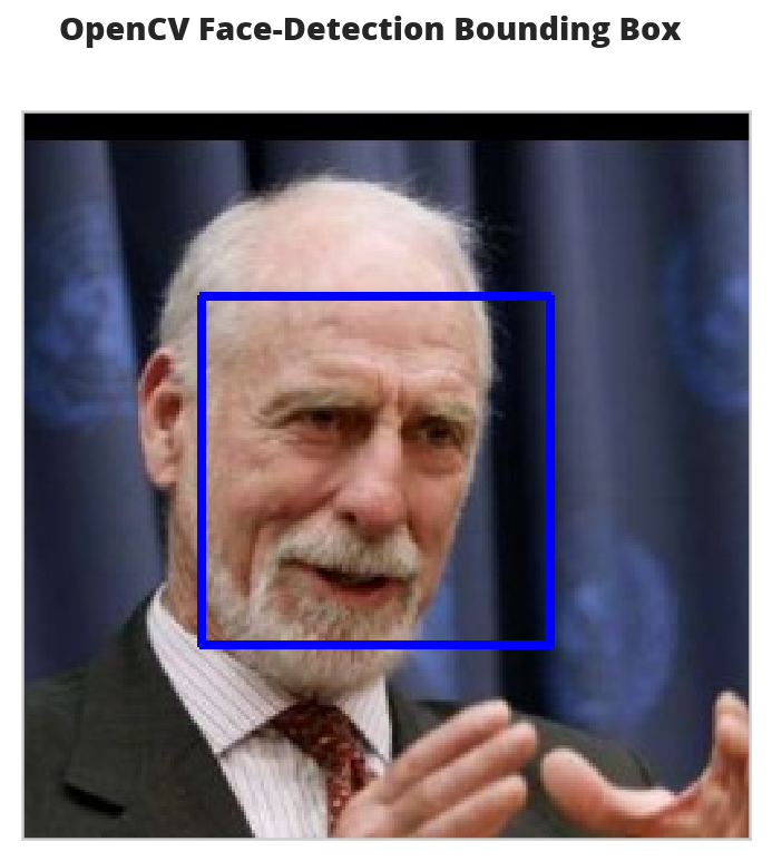
face_bounded.png

Write a Human Face Detector

Now that we know how it works, we can use the OpenCV face-recognizer to tell us if the image has a human in it (because there will be at least one bounding-box).

# returns "True" if face is detected in image stored at img_path
def face_detector(image_path: str) -> bool:
    """Detects human faces in an image

    Args:
     image_path: path to the image to check

    Returns:
     True if there was at least one face in the image
    """
    image = cv2.imread(image_path)
    gray = cv2.cvtColor(image, cv2.COLOR_BGR2GRAY)
    faces = face_cascade.detectMultiScale(gray)
    return len(faces) > 0

Assess the Human Face Detector

Here I'll check how well the face detector does using an F1 score. I'll also show some other metrics, but F1 is the single-value that I'll be focused on.

open_cv_scorer = human_scorer(face_detector)
open_cv_scorer()
Metric Value
Accuracy 0.94
Precision 0.90
Recall 0.99
Specificity 0.89
F1 0.94
Elapsed 0:02:42.880287

Overall the model seems to have done quite well. It was better at recall than specificity so it tended to classify some dogs as humans (around 11 %).

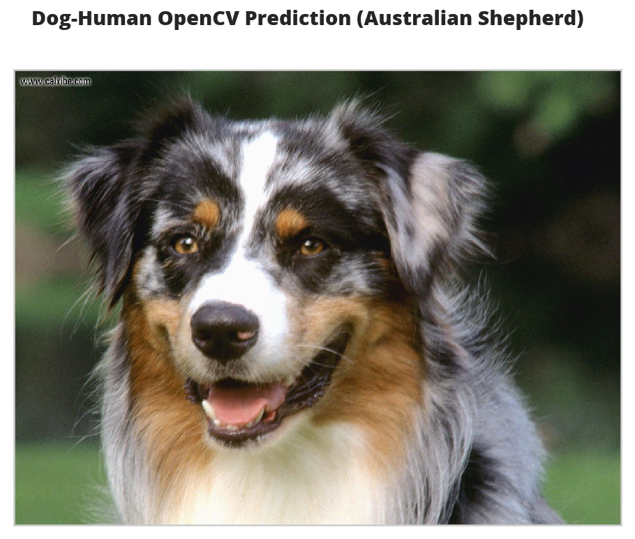
dogman_index = first_prediction(open_cv_scorer.false_image_predictions)
2: True

It looks like the third dog image was classified as a human by OpenCV.

source = dog_files_short[dogman_index]
name = get_name(source)
figure, axe = display_image(source,
                            "Dog-Human OpenCV Prediction ({})".format(name))
dog_man.png

I guess I can see where this might look like a human face. Maybe.

DLIB

I'm also going to test face_recognition, a python interface to dlib's facial recognition code. Unlike OpenCV, face_recognition doesn't require you to do the image-conversions before looking for faces.

Inspect an Image

image = face_recognition.load_image_file(sample_face)
locations = face_recognition.face_locations(image)
image = mpimage.imread(sample_face)
figure, axe = display_image(image, "dlib Face Recognition Bounding-Box", False)
top, right, bottom, left = locations[0]
width = right - left
height = top - bottom
rectangle = patches.Rectangle((top, right), width, height, fill=False)
patch = axe.add_patch(rectangle)

dlib_box.png

This box seems to be more tightly cropped than the Open CV version.

The Face Detecor

def face_recognition_check(image_path: str) -> bool:
    """This decides if an image has a face in it

    Args:
     image_path: path to an image
    Returns:
     True if there's at least one face in the image
    """
    image = face_recognition.load_image_file(str(image_path))
    locations = face_recognition.face_locations(image)
    return len(locations) > 0

Assess the Face Detector

dlib_dog_humans = human_scorer(face_recognition_check)
dlib_dog_humans()
Metric Value
Accuracy 0.95
Precision 0.92
Recall 1.00
Specificity 0.91
F1 0.96
Elapsed 0:09:28.752909

Dlib took around four times as long to run as OpenCV did, but did better overall.

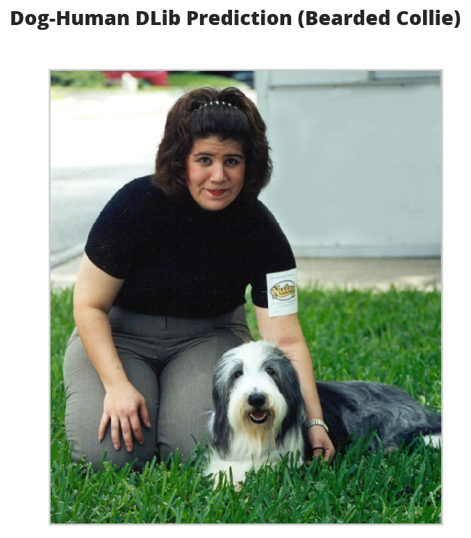
dlib_dog_human_index = first_prediction(dlib_dog_humans.false_image_predictions)
5: True

The dlib model didn't have a false positive for the third image like the OpenCV model did, but it did get the sixth image wrong.

source = dog_files_short[dlib_dog_human_index]
name = get_name(source)
figure, axe = display_image(source,
                            "Dog-Human DLib Prediction ({})".format(name))
dlib_dog_man.png

These photos with humans and dogs in them seem problematic.

face_recognition provides another model based on a CNN that I wanted to try but it gives me out-of-memory errors so I'll have to save that for later.

A Dog Detector

Now I'll take two pre-trained CNNs and use transfer learning to have them detect dogs in images.

A Dog Detector Function

If you look at the imagenet dictionary, you'll see that the categories for dogs have indices from 151 to 268, so without altering our models we can check if an image is a dog by seeing if they classify the image within this range of values.

DOG_LOWER, DOG_UPPER = 150, 260
def dog_detector(img_path: Path, predictor: object):
    """Predicts if the image is a dog

    Args:
     img_path: path to image file
     predictor: callable that maps the image to an ID

    Returns:
     is-dog: True if the image contains a dog
    """
    return DOG_LOWER < predictor(img_path) < DOG_UPPER

The VGG-16 Model

I'm going to use a VGG-16 model, along with weights that have been trained on ImageNet, a data set containing objects from one of 1000 categories.

Pytorch comes with a VGG 16 model built-in so we just have to declare it with the pretrained=True argument to download and load it.

timer.start()
VGG16 = models.vgg16(pretrained=True)
VGG16.eval()
VGG16.to(device)
MODELS.append(VGG16)
timer.end()
Started: 2019-01-13 14:43:39.512124
Ended: 2019-01-13 14:44:07.819057
Elapsed: 0:00:28.306933

Note: The first time you run this it has to download the state dictionary so it will take much longer than it would once you've run it at least once.

Making Predictions With the VGG 16 Model

In order to use the images with our model we have to run them through a transform. Even then, the forward-pass expects you to pass it a batch, not a single image, so you have to add an extra (fourth) dimension to the images to represent the batch. I found out how to fix the dimensions (using unsqueeze to add an empty dimension) from this blog post.

This next block sets up the transforms. Each pre-trained model expects a specific image-size for the inputs. In this case the VGG16 model expects a 224 x 224 image (which is why I set the IMAGE_SIZE to 224).

The images also have to be normalized using a specific set of means and standard deviations, but since pytorch uses the same ones for all the models I defined them at the top of this document because I'll be using them later for the inception model as well.

IMAGE_SIZE = 224
IMAGE_HALF_SIZE = IMAGE_SIZE//2

vgg_transform = transforms.Compose([transforms.Resize(255),
                                    transforms.CenterCrop(IMAGE_SIZE),
                                    transforms.ToTensor(),
                                    transforms.Normalize(MEANS,
                                                         DEVIATIONS)])

VGG16 Predict

This is a function to predict what class an image is.

def VGG16_predict(img_path: str) -> int:
    '''
    Uses a pre-trained VGG-16 model to obtain the index corresponding to 
    predicted ImageNet class for image at specified path

    Args:
        img_path: path to an image

    Returns:
        Index corresponding to VGG-16 model's prediction
    '''
    image = Image.open(str(img_path))
    image = vgg_transform(image).unsqueeze(0).to(device)
    output = VGG16(image)
    probabilities = torch.exp(output)
    top_probability, top_class = probabilities.topk(1, dim=1)
    return top_class.item()

Let's see what the model predicts for an image.

path = numpy.random.choice(dog_files_short)
print(path)
classification = VGG16_predict(path)
print(imagenet[classification])
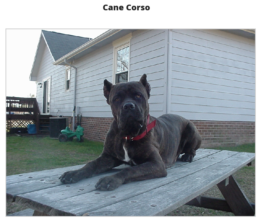
/home/hades/data/datasets/dog-breed-classification/dogImages/valid/044.Cane_corso/Cane_corso_03122.jpg
American Staffordshire terrier, Staffordshire terrier, American pit bull terrier, pit bull terrier

Our classifier recognizes that the image is a dog, but thinks that it's a Terrire, not a Cane Corso. Here's what it saw.

name = get_name(path)
figure, axe = display_image(path, name)
vgg_misclassified.png

And this is what it thought it was (a bull-mastiff).

american_staffordshire_terrier.jpg

Assess the Dog Detector

Now, as with the human face-detectors, I'll calculate some metrics to see how the VGG16 dog-detector does.

dog_scorer = partial(F1Scorer, true_images=dog_files_short,
                     false_images=human_files_short)
vgg_predictor = partial(dog_detector, predictor=VGG16_predict)
 vgg_scorer = dog_scorer(vgg_predictor)
 vgg_scorer()
Metric Value
Accuracy 0.95
Precision 0.99
Recall 0.92
Specificity 0.99
F1 0.95
Elapsed 0:02:37.257690

Unlike the face-detectors, the VGG16 dog detector did better at avoiding false-positives than it did at detecting dogs.

Inception

The previous detector used the VGG 16 model, but now I'll try the Inception-v3 model, which was designed to use less resources than the VGG model, to do some dog-detection.

 timer.start()
 inception = models.inception_v3(pretrained=True)
 inception.to(device)
 inception.eval()
 MODELS.append(inception)
 timer.end()
Started: 2019-01-13 18:45:27.709998
Ended: 2019-01-13 18:45:31.775443
Elapsed: 0:00:04.065445

Making a Prediction

This was my original dog detector using the Inception model, but when I tried it out it raised an error. See the next section for more information and the fix.

 def inception_predicts(image_path: str) -> int:
     """Predicts the category of the image

     Args:
      image_path: path to the image file

     Returns:
      classification: the resnet ID for the image
     """
     image = Image.open(str(image_path))
     image = vgg_transform(image).unsqueeze(0).to(device)
     output = inception(image)
     probabilities = torch.exp(output)
     top_probability, top_class = probabilities.topk(1, dim=1)
     return top_class.item()

Troubleshooting the Error

The inception_predicts is throwing a Runtime Error saying that the sizes must be non-negative. I'll grab a file here to check it out.

 for path in dog_files_short:
     try:
         prediction = inception_predicts(path)
     except RuntimeError as error:
         print(error)
         print(path)
         break
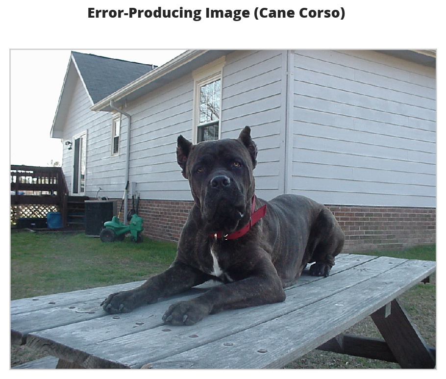
Given input size: (2048x5x5). Calculated output size: (2048x0x0). Output size is too small at /pytorch/aten/src/THCUNN/generic/SpatialAveragePooling.cu:63
/home/hades/data/datasets/dog-breed-classification/dogImages/valid/044.Cane_corso/Cane_corso_03122.jpg

So this dog raised an error, let's see what it looks like.

 name = get_name(path)
 figure, axe = display_image(path, "Error-Producing Image ({})".format(name))
inception_error.png

  • Why did this raise an error?

    I couldn't find anyplace where pytorch documents it, but if you look at the source code you can see that they are expecting an image size of 299 pixels, so we need a diferent transform from that used by the VGG model.

     INCEPTION_IMAGE_SIZE = 299
     inception_transforms = transforms.Compose([
         transforms.Resize(INCEPTION_IMAGE_SIZE),
         transforms.CenterCrop(INCEPTION_IMAGE_SIZE),
         transforms.ToTensor(),
         transforms.Normalize(MEANS,
                              DEVIATIONS)])
    

    Now try it again with the new transforms.

    def inception_predicts_two(image_path: str) -> int:
        """Predicts the category of the image
    
        Args:
         image_path: path to the image file
    
        Returns:
         classification: the resnet ID for the image
        """
        image = Image.open(str(image_path))
        image = inception_transforms(image).unsqueeze(0).to(device)
        output = inception(image)
        probabilities = torch.exp(output)
        top_probability, top_class = probabilities.topk(1, dim=1)
        return top_class.item()
    

    Does this fix it?

The Score

inception_predictor = partial(dog_detector, predictor=inception_predicts_two)
inception_scorer = dog_scorer(inception_predictor)
inception_scorer()
Metric Value
Accuracy 0.95
Precision 0.99
Recall 0.91
Specificity 0.99
F1 0.95
Elapsed 0:03:00.836240

The inception had a little more false positives but also more true positives so in the end it came up about the same on the F1 score as the VGG 16 model. They both took about the same amount of time.

inception_human_dog = first_prediction(inception_scorer.false_image_predictions)
34: True
figure, axe = pyplot.subplots()
source = human_files_short[inception_human_dog]
name = " ".join(
    os.path.splitext(
        os.path.basename(source))[0].split("_")[:-1]).title()
figure.suptitle("Human-Dog Inception Prediction ({})".format(
    name), weight="bold")
image = Image.open(source)
image = axe.imshow(image)
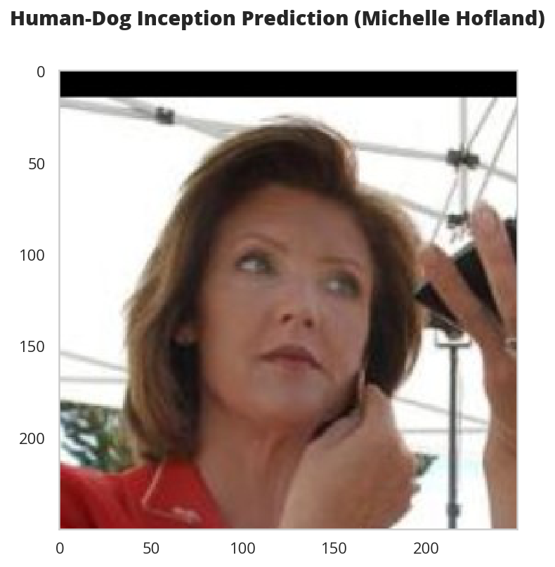
inception_man_dog.png

Combine The Detectors

Since jupyter (or org-babel) lets you run cells out of sequence I've spent too much time chasing bugs that weren't really bugs, I just hadn't run the right cell. To try and ameliorate that I'm going to use class-based code for the actual implementations.

The Dog Detector

The Dog Detector builds the parts of the deep learning model that are needed to check if there are dogs in the image.

class DogDetector:
    """Detects dogs

    Args:
     model_definition: definition for the model
     device: where to run the model (CPU or CUDA)
     image_size: what to resize the file to (depends on the model-definition)
     means: mean for each channel
     deviations: standard deviation for each channel
     dog_lower_bound: index below where dogs start
     dog_upper_bound: index above where dogs end
    """
    def __init__(self,
                 model_definition: nn.Module=models.inception_v3,
                 image_size: int=INCEPTION_IMAGE_SIZE,
                 means: list=MEANS,
                 deviations = DEVIATIONS,
                 dog_lower_bound: int=DOG_LOWER,
                 dog_upper_bound: int=DOG_UPPER,
                 device: torch.device=None) -> None:
        self.model_definition = model_definition
        self.image_size = image_size
        self.means = means
        self.deviations = deviations
        self.dog_lower_bound = dog_lower_bound
        self.dog_upper_bound = dog_upper_bound
        self._device = device
        self._model = None
        self._transform = None
        return

    @property
    def device(self) -> torch.device:
        """The device to add the model to"""
        if self._device is None:
            self._device = torch.device("cuda"
                                        if torch.cuda.is_available()
                                        else "cpu")
        return self._device

    @property
    def model(self) -> nn.Module:
        """Build the model"""
        if self._model is None:
            self._model = self.model_definition(pretrained=True)
            self._model.to(self.device)
            self._model.eval()
        return self._model

    @property
    def transform(self) -> transforms.Compose:
        """The transformer for the image data"""
        if self._transform is None:
            self._transform = transforms.Compose([
                transforms.Resize(self.image_size),
                transforms.CenterCrop(self.image_size),
                transforms.ToTensor(),
                transforms.Normalize(self.means,
                                     self.deviations)])
        return self._transform

    def __call__(self, image_path: str) -> bool:
        """Checks if there is a dog in the image"""
        image = Image.open(str(image_path))
        image = self.transform(image).unsqueeze(0).to(self.device)
        output = self.model(image)
        probabilities = torch.exp(output)
        _, top_class = probabilities.topk(1, dim=1)
        return self.dog_lower_bound < top_class.item() < self.dog_upper_bound

The Species Detector

The Species Detector holds the human and dog detectors.

class SpeciesDetector:
    """Detect dogs and humans

    Args:
     device: where to put the dog-detecting model
    """
    def __init__(self, device: torch.device=None) -> None:
        self.device = device
        self._dog_detector = None
        return

    @property
    def dog_detector(self) -> DogDetector:
        """Neural Network dog-detector"""
        if self._dog_detector is None:
            self._dog_detector = DogDetector(device=self.device)
        return self._dog_detector

    def is_human(self, image_path: str) -> bool:
        """Checks if the image is a human

        Args:
         image_path: path to the image

        Returns:
         True if there is a human face in the image
        """
        image = face_recognition.load_image_file(str(image_path))
        faces = face_recognition.face_locations(image)
        return len(faces) > 0

    def is_dog(self, image_path: str) -> bool:        
        """Checks if there is a dog in the image"""
        return self.dog_detector(image_path)

A Dog Breed Classifier

Although the Inception model does do some classification of dogs, we want an even more fine-tuned model. First I'm going to try to build a naive CNN from scratch, then I'm going to use the Inception model and transfer learning to build a better classifier.

A Naive Model

The Data Transformers

For the naive model I'm going to use the image-size the VGG model uses (the original VGG paper describes the input as being 224 x 224). No particular reason except I've worked with that size before so I think it might make troubleshooting a little easier. The Resize transform scales the image so that the smaller edge matches the size we give it. I found out the hard way that not all the input images are square so we need to then crop them back to the right size after scaling.

Here's the training tranforms:

For testing and using:

For both:

IMAGE_SIZE = 224
IMAGE_HALF_SIZE = IMAGE_SIZE//2

train_transform = transforms.Compose([
    transforms.RandomRotation(30),
    transforms.RandomResizedCrop(IMAGE_SIZE),
    transforms.RandomHorizontalFlip(),
    transforms.ToTensor(),
    transforms.Normalize(MEANS,
                         DEVIATIONS)])

test_transform = transforms.Compose([transforms.Resize(255),
                                      transforms.CenterCrop(IMAGE_SIZE),
                                      transforms.ToTensor(),
                                      transforms.Normalize(MEANS,
                                                           DEVIATIONS)])

Load the Data

training = datasets.ImageFolder(root=str(dog_paths.training.folder),
                                transform=train_transform)
validation = datasets.ImageFolder(root=str(dog_paths.validation.folder),
                                  transform=test_transform)
testing = datasets.ImageFolder(root=str(dog_paths.testing.folder),
                               transform=test_transform)

Build the Batch Loaders

BATCH_SIZE = 35
WORKERS = 0

train_batches = torch.utils.data.DataLoader(training, batch_size=BATCH_SIZE,
                                            shuffle=True, num_workers=WORKERS)
validation_batches = torch.utils.data.DataLoader(
    validation, batch_size=BATCH_SIZE, shuffle=True, num_workers=WORKERS)
test_batches = torch.utils.data.DataLoader(
    testing, batch_size=BATCH_SIZE, shuffle=True, num_workers=WORKERS)

loaders_scratch = dict(train=train_batches,
                       validate=validation_batches,
                       test=test_batches)

The Network

This is only going to be a three-layer model. I started out trying to make a really big one but between the computation time and running out of memory I decided to limit the scope since the transfer model is the real one I want anyway, this is just for practice. The first block defines the parameters for the network.

LAYER_ONE_OUT = 16
LAYER_TWO_OUT = LAYER_ONE_OUT * 2
LAYER_THREE_OUT = LAYER_TWO_OUT * 2

KERNEL = 3
PADDING = 1
FULLY_CONNECTED_OUT = 500

This next block does one pass through what the network is going to be doing so I can make sure the inputs and outputs are the correct size.

conv_1 = nn.Conv2d(3, LAYER_ONE_OUT, KERNEL, padding=PADDING)
conv_2 = nn.Conv2d(LAYER_ONE_OUT, LAYER_TWO_OUT, KERNEL, padding=PADDING)
conv_3 = nn.Conv2d(LAYER_TWO_OUT, LAYER_THREE_OUT, KERNEL, padding=PADDING)

pool = nn.MaxPool2d(2, 2)
dropout = nn.Dropout(0.25)

fully_connected_1 = nn.Linear((IMAGE_HALF_SIZE//4)**2 * LAYER_THREE_OUT, FULLY_CONNECTED_OUT)
fully_connected_2 = nn.Linear(FULLY_CONNECTED_OUT, dog_paths.breed_count)

dataiter = iter(loaders_scratch['train'])
images, labels = dataiter.next()

x = pool(F.relu(conv_1(images)))
print(x.shape)
assert x.shape == torch.Size([BATCH_SIZE, 16, IMAGE_HALF_SIZE, IMAGE_HALF_SIZE])

x = pool(F.relu(conv_2(x)))
print(x.shape)
assert x.shape == torch.Size([BATCH_SIZE, LAYER_TWO_OUT, IMAGE_HALF_SIZE//2, IMAGE_HALF_SIZE//2])

x = pool(F.relu(conv_3(x)))
print(x.shape)
assert x.shape == torch.Size([BATCH_SIZE, LAYER_THREE_OUT, IMAGE_HALF_SIZE//4, IMAGE_HALF_SIZE//4])

x = x.view(-1, ((IMAGE_HALF_SIZE//4)**2) * LAYER_THREE_OUT)
print(x.shape)
x = fully_connected_1(x)
print(x.shape)
x = fully_connected_2(x)
print(x.shape)
torch.Size([10, 16, 112, 112])
torch.Size([10, 32, 56, 56])
torch.Size([10, 64, 28, 28])
torch.Size([10, 50176])
torch.Size([10, 500])
torch.Size([10, 133])

The Class

This is the actual implementation based on the previous code.

class NaiveNet(nn.Module):
    """Naive Neural Network to classify dog breeds"""
    def __init__(self) -> None:
        super().__init__()
        self.conv1 = nn.Conv2d(3, LAYER_ONE_OUT,
                               KERNEL, padding=PADDING)
        self.conv2 = nn.Conv2d(LAYER_ONE_OUT, LAYER_TWO_OUT,
                               KERNEL, padding=PADDING)
        self.conv3 = nn.Conv2d(LAYER_TWO_OUT, LAYER_THREE_OUT,
                               KERNEL, padding=PADDING)
        # max pooling layer
        self.pool = nn.MaxPool2d(2, 2)
        # linear layer
        self.fc1 = nn.Linear((IMAGE_HALF_SIZE//4)**2 * LAYER_THREE_OUT, FULLY_CONNECTED_OUT)
        self.fc2 = nn.Linear(FULLY_CONNECTED_OUT, BREEDS)
        # dropout layer (p=0.25)
        self.dropout = nn.Dropout(0.25)
        return


    def forward(self, x: torch.Tensor) -> torch.Tensor:
        """The forward pass method

        Args:
         x: a n x 224 x 224 x 3 tensor

        Returns:
         tensor of probabilities
        """
        x = self.pool(F.relu(self.conv1(x)))
        x = self.pool(F.relu(self.conv2(x)))
        x = self.pool(F.relu(self.conv3(x)))

        x = x.view(-1, (IMAGE_HALF_SIZE//4)**2 * LAYER_THREE_OUT)
        x = self.dropout(x)

        x = self.dropout(F.relu(self.fc1(x)))
        x = self.fc2(x)        
        return x
naive_model = NaiveNet()
naive_model.to(device)
MODELS.append(naive_model)

The Loss Function and Optimizer

For loss measurement I'm going to use Cross Entropy Loss and Stochastic Gradient Descent for backward propagation.

criterion_scratch = nn.CrossEntropyLoss()
optimizer_scratch = optimizer.SGD(naive_model.parameters(),
                                  lr=0.001,
                                  momentum=0.9)

Train and Validate the Model

  • The Trainer

    Another class to try and get everything bundled into one place.

    class Trainer:
        """Trains, validates, and tests the model
    
        Args:
         training_batches: batch-loaders for training
         validation_batches: batch-loaders for validation
         testing_batches: batch-loaders for testing
         model: the network to train
         model_path: where to save the best model
         optimizer: the gradient descent object
         criterion: object to do backwards propagation
         device: where to put the data (cuda or cpu)
         epochs: number of times to train on the data set
         epoch_start: number to start the epoch count with
         load_model: whether to load the model from a file
         beep: whether timer should emit sounds
         is_inception: expecte two outputs in training
        """
        def __init__(self,
                     training_batches: torch.utils.data.DataLoader,
                     validation_batches: torch.utils.data.DataLoader,
                     testing_batches: torch.utils.data.DataLoader,
                     model: nn.Module,
                     model_path: Path,
                     optimizer: optimizer.SGD,
                     criterion: nn.CrossEntropyLoss,
                     device: torch.device=None,
                     epochs: int=10,
                     epoch_start: int=1,
                     is_inception: bool=False,
                     load_model: bool=False,
                     beep: bool=False) -> None:
            self.training_batches = training_batches
            self.validation_batches = validation_batches
            self.testing_batches = testing_batches
            self.model = model
            self.model_path = model_path
            self.optimizer = optimizer
            self.criterion = criterion
            self.epochs = epochs
            self.is_inception = is_inception
            self.beep = beep
            self._epoch_start = None
            self.epoch_start = epoch_start
            self.load_model = load_model
            self._timer = None
            self._epoch_end = None
            self._device = device
            return
    
        @property
        def epoch_start(self) -> int:
            """The number to start the epoch count"""
            return self._epoch_start
    
        @epoch_start.setter
        def epoch_start(self, new_start: int) -> None:
            """Sets the epoch start, removes the epoch end"""
            self._epoch_start = new_start
            self._epoch_end = None
            return
    
        @property
        def device(self) -> torch.device:
            """The device to put the data on"""
            if self._device is None:
                self._device = torch.device("cuda" if torch.cuda.is_available()
                                            else "cpu")
            return self._device
    
        @property
        def epoch_end(self) -> int:
            """the end of the epochs (not inclusive)"""
            if self._epoch_end is None:
                self._epoch_end = self.epoch_start + self.epochs
            return self._epoch_end
    
        @property
        def timer(self) -> Timer:
            """something to emit times"""
            if self._timer is None:
                self._timer = Timer(beep=self.beep)
            return self._timer
    
        def forward(self, batches: torch.utils.data.DataLoader,
                    training: bool) -> tuple:
            """runs the forward pass
    
            Args:
             batches: data-loader
             training: if true, runs the training, otherwise validates
            Returns:
             tuple: loss, correct, total
            """
            forward_loss = 0
            correct = 0
    
            if training:
                self.model.train()
            else:
                self.model.eval()
            for data, target in batches:
                data, target = data.to(self.device), target.to(self.device)
                if training:
                    self.optimizer.zero_grad()
                if training and self.is_inception:
                    # throw away the auxiliary output
                    output, _ = self.model(data)
                output = self.model(data)
                loss = self.criterion(output, target)
                if training:
                    loss.backward()
                    self.optimizer.step()
                forward_loss += loss.item() * data.size(0)
    
                predictions = output.data.max(1, keepdim=True)[1]
                correct += numpy.sum(
                    numpy.squeeze(
                        predictions.eq(
                            target.data.view_as(predictions))).cpu().numpy())
            forward_loss /= len(batches.dataset)
            return forward_loss, correct, len(batches.dataset)
    
        def train(self) -> tuple:
            """Runs the training
    
            Returns:
             training loss, correct, count
            """
            return self.forward(batches=self.training_batches, training=True)
    
        def validate(self) -> tuple:
            """Runs the validation
    
            Returns:
             validation loss, correct, count
            """
            return self.forward(batches=self.validation_batches, training=False)
    
        def test(self) -> None:
            """Runs the testing
    
            """
            self.timer.start()
            self.model.load_state_dict(torch.load(self.model_path))
            loss, correct, total = self.forward(batches=self.testing_batches,
                                                training=False)
            print("Test Loss: {:.3f}".format(loss))
            print("Test Accuracy: {:.2f} ({}/{})".format(100 * correct/total,
                                                         correct, total))
            self.timer.end()
            return
    
        def train_and_validate(self):
            """Trains and Validates the model
            """
            validation_loss_min = numpy.Inf
            for epoch in range(self.epoch_start, self.epoch_end):
                self.timer.start()
                training_loss, training_correct, training_count = self.train()
                (validation_loss, validation_correct,
                 validation_count) = self.validate()
                self.timer.end()
                print(("Epoch: {}\t"
                       "Training - Loss: {:.2f}\t"
                       "Accuracy: {:.2f}\t"
                       "Validation - Loss: {:.2f}\t"
                       "Accuracy: {:.2f}").format(
                           epoch,
                           training_loss,
                           training_correct/training_count,
                           validation_loss,
                           validation_correct/validation_count,
                    ))
    
                if validation_loss < validation_loss_min:
                    print(
                        ("Validation loss decreased ({:.6f} --> {:.6f}). "
                         "Saving model ...").format(
                             validation_loss_min,
                             validation_loss))
                    torch.save(self.model.state_dict(), self.model_path)
                    validation_loss_min = validation_loss
            return
    
        def __call__(self) -> None:
            """Trains, Validates, and Tests the model"""
            if self.load_model and self.model_path.is_file():
                self.model.load_state_dict(torch.load(self.model_path))
            print("Starting Training")
            self.timer.start()
            self.train_and_validate()
            self.timer.end()
            print("\nStarting Testing")
            self.test()
            return
    

Broken Images

I noted at the beginning of the notebook that at least one of the images is raising an OSError:

OSError: image file is truncated (150 bytes not processed)

This is the part of the notebook where I originally found out what was going on (because it kept crashing during training).

timer.start()
broken = None
for image in dog_files:
    try:
        opened = Image.open(image)
        opened.convert("RGB")
    except OSError as error:
        print("{}: {}".format(error, image))
        broken = image
timer.end()
image file is truncated (150 bytes not processed): /home/hades/datasets/dog-breed-classification/dogImages/train/098.Leonberger/Leonberger_06571.jpg
Ended: 2018-12-30 15:10:19.141003
Elapsed: 0:02:29.804925
figure, axe = pyplot.subplots()
name = " ".join(broken.name.split("_")[:-1]).title()
figure.suptitle("Truncated Image ({})".format(name), weight="bold")
image = Image.open(broken)
axe_image = axe.imshow(image)
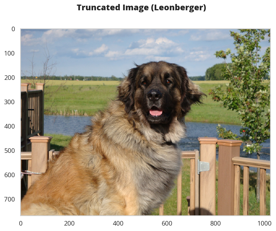
truncated_dog.png

I got the solution from this Stack Overflow post, I don't know why but the image seems to be missing some pixels or something. Oh, well. The key to making it work:

ImageFile.LOAD_TRUNCATED_IMAGES = True

Train the Model

NAIVE_PATH = MODEL_PATH.folder.joinpath("model_scratch.pt")
scratch_log = Tee(log_name="scratch_train.log")

Test the Model

def test(test_batches: torch.utils.data.DataLoader,
         model: nn.Module,
         criterion: nn.CrossEntropyLoss) -> None:
    """Test the model

    Args:
     test_batches: batch loader of test images
     model: the network to test
     criterion: calculator for the loss
    """
    test_loss = 0.
    correct = 0.
    total = 0.

    model.eval()
    for data, target in test_batches:
        data, target = data.to(device), target.to(device)
        output = model(data)
        loss = criterion(output, target)
        test_loss += loss.item() * data.size(0)
        # convert output probabilities to predicted class
        predictions = output.data.max(1, keepdim=True)[1]
        # compare predictions to true label
        correct += numpy.sum(
            numpy.squeeze(
                predictions.eq(
                    target.data.view_as(predictions))).cpu().numpy())
        total += data.size(0)
    test_loss /= len(test_batches.dataset)
    print('Test Loss: {:.6f}\n'.format(test_loss))
    print('\nTest Accuracy: %2d%% (%2d/%2d)' % (
        100. * correct / total, correct, total))
    return

Train and Test

def train_and_test(train_batches: torch.utils.data.DataLoader,
                   validate_batches: torch.utils.data.DataLoader,
                   test_batches: torch.utils.data.DataLoader,
                   model: nn.Module,
                   model_path: Path,
                   optimizer: optimizer.SGD,
                   criterion: nn.CrossEntropyLoss,
                   epochs: int=10,
                   epoch_start: int=1,
                   load_model: bool=False) -> None:
    """Trains and Tests the Model

    Args:
     train_batches: batch-loaders for training
     validate_batches: batch-loaders for validation
     test_batches: batch-loaders for testing
     model: the network to train
     model_path: where to save the best model
     optimizer: the gradient descent object
     criterion: object to do backwards propagation
     epochs: number of times to train on the data set
     epoch_start: number to start the epoch count with
     load_model: whether to load the model from a file
    """
    if load_model and model_path.is_file():
        model.load_state_dict(torch.load(model_path))
    print("Starting Training")
    timer.start()
    model_scratch = train(epochs=epochs,
                          epoch_start=epoch_start,
                          train_batches=train_batches,
                          validation_batches=validate_batches,
                          model=model,
                          optimizer=optimizer, 
                          criterion=criterion,
                          save_path=model_path)
    timer.end()
    # load the best model
    model.load_state_dict(torch.load(model_path))
    print("Starting Testing")
    timer.start()
    test(test_batches, model, criterion)
    timer.end()
    return

Train the Model

When I originally wrote this I was using this functional-style of training and testing, which was hard to use, but since it's so expensive to train the model (in terms of time, and to some degree server cost) I'm not going to re-do it so the code here looks a little different from the one I used for the transfer model.

model_path = DataPathTwo(
    folder_key="MODELS",
    filename="model_scratch.pt")
assert model_path.folder.is_dir()
train_and_test(epochs=10,
               train_batches=loaders_scratch["train"],
               validate_batches=loaders_scratch["validate"],
               test_batches=loaders_scratch["test"],
               model=model_scratch,
               optimizer=optimizer_scratch, 
               criterion=criterion_scratch,
               epoch_start=0,
               model_path=model_path.from_folder,
               load_model=False)
next_start = 11
Starting Training
Ended: 2019-01-01 16:35:14.192989
Elapsed: 0:03:23.778459
Epoch: 0        Training Loss: 3.946975         Validation Loss: 3.758706
Validation loss decreased (inf --> 3.758706). Saving model ...
Ended: 2019-01-01 16:38:39.497147
Elapsed: 0:03:24.517456
Epoch: 1        Training Loss: 3.880984         Validation Loss: 3.695643
Validation loss decreased (3.758706 --> 3.695643). Saving model ...
Ended: 2019-01-01 16:42:04.190248
Elapsed: 0:03:23.903292
Epoch: 2        Training Loss: 3.870710         Validation Loss: 3.718353
Ended: 2019-01-01 16:45:28.479552
Elapsed: 0:03:23.718292
Epoch: 3        Training Loss: 3.836664         Validation Loss: 3.740289
Ended: 2019-01-01 16:48:53.605419
Elapsed: 0:03:24.555708
Epoch: 4        Training Loss: 3.819701         Validation Loss: 3.659244
Validation loss decreased (3.695643 --> 3.659244). Saving model ...
Ended: 2019-01-01 16:52:33.198097
Elapsed: 0:03:38.805586
Epoch: 5        Training Loss: 3.778872         Validation Loss: 3.756706
Ended: 2019-01-01 16:56:16.822584
Elapsed: 0:03:43.055469
Epoch: 6        Training Loss: 3.752981         Validation Loss: 3.679196
Ended: 2019-01-01 16:59:42.861936
Elapsed: 0:03:25.469331
Epoch: 7        Training Loss: 3.730930         Validation Loss: 3.608311
Validation loss decreased (3.659244 --> 3.608311). Saving model ...
Ended: 2019-01-01 17:03:10.958002
Elapsed: 0:03:27.305644
Epoch: 8        Training Loss: 3.705110         Validation Loss: 3.636201
Ended: 2019-01-01 17:06:38.939991
Elapsed: 0:03:27.412824
Epoch: 9        Training Loss: 3.665519         Validation Loss: 3.595410
Validation loss decreased (3.608311 --> 3.595410). Saving model ...
Ended: 2019-01-01 17:06:39.733176
Elapsed: 0:03:28.206009
Starting Testing
Test Loss: 3.642843


Test Accuracy: 14% (125/836)
Ended: 2019-01-01 17:07:11.142926
Elapsed: 0:00:30.815650

Hmm, seems suspiciously good all of a sudden. It looks like my GPU is faster than paper space's, too..

train_and_test(epochs=10,
               train_batches=loaders_scratch["train"],
               validate_batches=loaders_scratch["validate"],
               test_batches=loaders_scratch["test"],
               model=model_scratch,
               optimizer=optimizer_scratch, 
               criterion=criterion_scratch,
               epoch_start=next_start,
               model_path=model_path.from_folder,
               load_model=True)
next_start = 21
Starting Training
Ended: 2019-01-01 17:29:46.425198
Elapsed: 0:03:40.954699
Epoch: 0        Training Loss: 3.662736         Validation Loss: 3.631118
Validation loss decreased (inf --> 3.631118). Saving model ...
Ended: 2019-01-01 17:33:12.797754
Elapsed: 0:03:25.528229
Epoch: 1        Training Loss: 3.612436         Validation Loss: 3.610919
Validation loss decreased (3.631118 --> 3.610919). Saving model ...
Ended: 2019-01-01 17:36:49.466848
Elapsed: 0:03:35.831733
Epoch: 2        Training Loss: 3.612902         Validation Loss: 3.590953
Validation loss decreased (3.610919 --> 3.590953). Saving model ...
Ended: 2019-01-01 17:40:17.511898
Elapsed: 0:03:27.192943
Epoch: 3        Training Loss: 3.564542         Validation Loss: 3.566365
Validation loss decreased (3.590953 --> 3.566365). Saving model ...
Ended: 2019-01-01 17:43:45.639219
Elapsed: 0:03:27.309572
Epoch: 4        Training Loss: 3.551703         Validation Loss: 3.608934
Ended: 2019-01-01 17:47:32.854824
Elapsed: 0:03:46.646159
Epoch: 5        Training Loss: 3.542706         Validation Loss: 3.533696
Validation loss decreased (3.566365 --> 3.533696). Saving model ...
Ended: 2019-01-01 17:51:02.330525
Elapsed: 0:03:28.506819
Epoch: 6        Training Loss: 3.532894         Validation Loss: 3.531388
Validation loss decreased (3.533696 --> 3.531388). Saving model ...
Ended: 2019-01-01 17:54:25.844725
Elapsed: 0:03:22.697779
Epoch: 7        Training Loss: 3.482241         Validation Loss: 3.564429
Ended: 2019-01-01 17:57:48.563069
Elapsed: 0:03:22.148237
Epoch: 8        Training Loss: 3.485189         Validation Loss: 3.624133
Ended: 2019-01-01 18:01:11.755236
Elapsed: 0:03:22.621310
Epoch: 9        Training Loss: 3.461059         Validation Loss: 3.594314
Ended: 2019-01-01 18:01:12.326268
Elapsed: 0:03:23.192342
Starting Testing
Test Loss: 3.537503


Test Accuracy: 16% (138/836)
Ended: 2019-01-01 18:01:42.764907
Elapsed: 0:00:29.747148
train_and_test(epochs=10,
               train_batches=loaders_scratch["train"],
               validate_batches=loaders_scratch["validate"],
               test_batches=loaders_scratch["test"],
               model=model_scratch,
               optimizer=optimizer_scratch, 
               criterion=criterion_scratch,
               epoch_start=next_start,
               model_path=model_path.from_folder,
               load_model=True)
next_start = 31
Starting Training
Ended: 2019-01-01 18:45:17.404562
Elapsed: 0:03:23.081286
Epoch: 21       Training Loss: 3.510303         Validation Loss: 3.555182
Validation loss decreased (inf --> 3.555182). Saving model ...
Ended: 2019-01-01 18:48:41.215171
Elapsed: 0:03:22.949288
Epoch: 22       Training Loss: 3.485824         Validation Loss: 3.570289
Ended: 2019-01-01 18:52:04.635395
Elapsed: 0:03:22.849569
Epoch: 23       Training Loss: 3.438656         Validation Loss: 3.543221
Validation loss decreased (3.555182 --> 3.543221). Saving model ...
Ended: 2019-01-01 18:55:28.409018
Elapsed: 0:03:22.980693
Epoch: 24       Training Loss: 3.387092         Validation Loss: 3.649569
Ended: 2019-01-01 18:58:51.555922
Elapsed: 0:03:22.576946
Epoch: 25       Training Loss: 3.381217         Validation Loss: 3.529994
Validation loss decreased (3.543221 --> 3.529994). Saving model ...
Ended: 2019-01-01 19:02:15.743200
Elapsed: 0:03:23.359857
Epoch: 26       Training Loss: 3.379801         Validation Loss: 3.514583
Validation loss decreased (3.529994 --> 3.514583). Saving model ...
Ended: 2019-01-01 19:05:40.243125
Elapsed: 0:03:23.700481
Epoch: 27       Training Loss: 3.334058         Validation Loss: 3.469988
Validation loss decreased (3.514583 --> 3.469988). Saving model ...
Ended: 2019-01-01 19:09:04.218270
Elapsed: 0:03:23.150903
Epoch: 28       Training Loss: 3.347201         Validation Loss: 3.456167
Validation loss decreased (3.469988 --> 3.456167). Saving model ...
Ended: 2019-01-01 19:12:27.711756
Elapsed: 0:03:22.677622
Epoch: 29       Training Loss: 3.320286         Validation Loss: 3.444669
Validation loss decreased (3.456167 --> 3.444669). Saving model ...
Ended: 2019-01-01 19:15:51.375887
Elapsed: 0:03:22.875358
Epoch: 30       Training Loss: 3.314001         Validation Loss: 3.460704
Ended: 2019-01-01 19:15:51.946497
Elapsed: 0:03:23.445968
Starting Testing
Test Loss: 3.492875


Test Accuracy: 17% (146/836)
Ended: 2019-01-01 19:16:10.729405
Elapsed: 0:00:18.109680
train_and_test(epochs=10,
               train_batches=loaders_scratch["train"],
               validate_batches=loaders_scratch["validate"],
               test_batches=loaders_scratch["test"],
               model=model_scratch,
               optimizer=optimizer_scratch, 
               criterion=criterion_scratch,
               epoch_start=next_start,
               model_path=model_path.from_folder,
               load_model=True)
next_start = 41
Starting Training
Ended: 2019-01-01 20:15:25.906348
Elapsed: 0:05:12.167322
Epoch: 31       Training Loss: 3.311046         Validation Loss: 3.446478
Validation loss decreased (inf --> 3.446478). Saving model ...
Ended: 2019-01-01 20:19:13.168084
Elapsed: 0:03:46.461085
Epoch: 32       Training Loss: 3.270769         Validation Loss: 3.550049
Ended: 2019-01-01 20:22:38.973465
Elapsed: 0:03:25.195274
Epoch: 33       Training Loss: 3.221883         Validation Loss: 3.489280
Ended: 2019-01-01 20:26:02.049299
Elapsed: 0:03:22.483931
Epoch: 34       Training Loss: 3.271723         Validation Loss: 3.507546
Ended: 2019-01-01 20:29:24.932614
Elapsed: 0:03:22.292605
Epoch: 35       Training Loss: 3.197156         Validation Loss: 3.475409
Ended: 2019-01-01 20:32:47.569786
Elapsed: 0:03:22.046763
Epoch: 36       Training Loss: 3.210177         Validation Loss: 3.477707
Ended: 2019-01-01 20:36:09.752175
Elapsed: 0:03:21.592504
Epoch: 37       Training Loss: 3.199346         Validation Loss: 3.577469
Ended: 2019-01-01 20:39:32.831340
Elapsed: 0:03:22.489048
Epoch: 38       Training Loss: 3.158563         Validation Loss: 3.442629
Validation loss decreased (3.446478 --> 3.442629). Saving model ...
Ended: 2019-01-01 20:42:56.293868
Elapsed: 0:03:22.664005
Epoch: 39       Training Loss: 3.152231         Validation Loss: 3.470943
Ended: 2019-01-01 20:46:18.983529
Elapsed: 0:03:22.098438
Epoch: 40       Training Loss: 3.124298         Validation Loss: 3.429367
Validation loss decreased (3.442629 --> 3.429367). Saving model ...
Ended: 2019-01-01 20:46:19.801009
Elapsed: 0:03:22.915918
Starting Testing
Test Loss: 3.348011


Test Accuracy: 21% (179/836)
Ended: 2019-01-01 20:46:42.494502
Elapsed: 0:00:22.094465
train_and_test(epochs=10,
               train_batches=loaders_scratch["train"],
               validate_batches=loaders_scratch["validate"],
               test_batches=loaders_scratch["test"],
               model=model_scratch,
               optimizer=optimizer_scratch, 
               criterion=criterion_scratch,
               epoch_start=next_start,
               model_path=model_path.from_folder,
               load_model=True)
next_start = 51
Starting Training
Ended: 2019-01-01 22:01:17.285699
Elapsed: 0:03:24.381614
Epoch: 41       Training Loss: 3.095166         Validation Loss: 3.418227
Validation loss decreased (inf --> 3.418227). Saving model ...
Ended: 2019-01-01 22:04:43.173252
Elapsed: 0:03:25.033381
Epoch: 42       Training Loss: 3.089258         Validation Loss: 3.419117
Ended: 2019-01-01 22:08:07.709900
Elapsed: 0:03:23.945667
Epoch: 43       Training Loss: 3.071535         Validation Loss: 3.433646
Ended: 2019-01-01 22:11:33.153513
Elapsed: 0:03:24.853880
Epoch: 44       Training Loss: 3.058665         Validation Loss: 3.454817
Ended: 2019-01-01 22:14:59.899762
Elapsed: 0:03:26.156530
Epoch: 45       Training Loss: 3.072674         Validation Loss: 3.494963
Ended: 2019-01-01 22:18:26.207188
Elapsed: 0:03:25.746042
Epoch: 46       Training Loss: 3.043788         Validation Loss: 3.430311
Ended: 2019-01-01 22:21:51.975083
Elapsed: 0:03:25.177310
Epoch: 47       Training Loss: 3.015571         Validation Loss: 3.382248
Validation loss decreased (3.418227 --> 3.382248). Saving model ...
Ended: 2019-01-01 22:25:18.237087
Elapsed: 0:03:25.403639
Epoch: 48       Training Loss: 2.972451         Validation Loss: 3.449296
Ended: 2019-01-01 22:28:44.315967
Elapsed: 0:03:25.498810
Epoch: 49       Training Loss: 2.989183         Validation Loss: 3.428347
Ended: 2019-01-01 22:32:10.738134
Elapsed: 0:03:25.832058
Epoch: 50       Training Loss: 2.966034         Validation Loss: 3.501775
Ended: 2019-01-01 22:32:11.326703
Elapsed: 0:03:26.420627
Starting Testing
Test Loss: 3.485910


Test Accuracy: 18% (156/836)
Ended: 2019-01-01 22:32:41.884173
Elapsed: 0:00:29.644028
train_and_test(epochs=10,
               train_batches=loaders_scratch["train"],
               validate_batches=loaders_scratch["validate"],
               test_batches=loaders_scratch["test"],
               model=model_scratch,
               optimizer=optimizer_scratch, 
               criterion=criterion_scratch,
               epoch_start=next_start,
               model_path=model_path.from_folder,
               load_model=True)
next_start = 61
Starting Training
Ended: 2019-01-01 22:39:53.821378
Elapsed: 0:04:15.535643
Epoch: 51       Training Loss: 3.024161         Validation Loss: 3.409968
Validation loss decreased (inf --> 3.409968). Saving model ...
Ended: 2019-01-01 22:43:47.462698
Elapsed: 0:03:52.776151
Epoch: 52       Training Loss: 2.979377         Validation Loss: 3.512004
Ended: 2019-01-01 22:47:35.580770
Elapsed: 0:03:47.528679
Epoch: 53       Training Loss: 2.983352         Validation Loss: 3.499196
Ended: 2019-01-01 22:50:58.662565
Elapsed: 0:03:22.501398
Epoch: 54       Training Loss: 2.944738         Validation Loss: 3.458440
Ended: 2019-01-01 22:54:21.531858
Elapsed: 0:03:22.279749
Epoch: 55       Training Loss: 2.921185         Validation Loss: 3.581930
Ended: 2019-01-01 22:57:44.017339
Elapsed: 0:03:21.925483
Epoch: 56       Training Loss: 2.928508         Validation Loss: 3.449956
Ended: 2019-01-01 23:01:06.668710
Elapsed: 0:03:22.061753
Epoch: 57       Training Loss: 2.887215         Validation Loss: 3.559204
Ended: 2019-01-01 23:04:29.439919
Elapsed: 0:03:22.181396
Epoch: 58       Training Loss: 2.909253         Validation Loss: 3.458249
Ended: 2019-01-01 23:07:51.804139
Elapsed: 0:03:21.803807
Epoch: 59       Training Loss: 2.864969         Validation Loss: 3.599446
Ended: 2019-01-01 23:11:14.184534
Elapsed: 0:03:21.789954
Epoch: 60       Training Loss: 2.820693         Validation Loss: 3.432991
Ended: 2019-01-01 23:11:14.775507
Elapsed: 0:03:22.380927
Starting Testing
Test Loss: 3.370016


Test Accuracy: 21% (176/836)
Ended: 2019-01-01 23:11:44.949942
Elapsed: 0:00:29.259563
next_start = 61
train_and_test(epochs=10,
               train_batches=loaders_scratch["train"],
               validate_batches=loaders_scratch["validate"],
               test_batches=loaders_scratch["test"],
               model=model_scratch,
               optimizer=optimizer_scratch, 
               criterion=criterion_scratch,
               epoch_start=next_start,
               model_path=model_path.from_folder,
               load_model=True)
next_start = 71
Starting Training
Ended: 2019-01-01 23:31:00.034455
Elapsed: 0:03:21.658811
Epoch: 61       Training Loss: 2.968425         Validation Loss: 3.469985
Validation loss decreased (inf --> 3.469985). Saving model ...
Ended: 2019-01-01 23:34:24.012685
Elapsed: 0:03:22.630721
Epoch: 62       Training Loss: 2.980103         Validation Loss: 3.449017
Validation loss decreased (3.469985 --> 3.449017). Saving model ...
Ended: 2019-01-01 23:37:47.137370
Elapsed: 0:03:22.315870
Epoch: 63       Training Loss: 2.945722         Validation Loss: 3.497296
Ended: 2019-01-01 23:41:09.932696
Elapsed: 0:03:22.226620
Epoch: 64       Training Loss: 2.940117         Validation Loss: 3.398626
Validation loss decreased (3.449017 --> 3.398626). Saving model ...
Ended: 2019-01-01 23:44:33.204607
Elapsed: 0:03:22.484337
Epoch: 65       Training Loss: 2.913762         Validation Loss: 3.465828
Ended: 2019-01-01 23:47:55.682608
Elapsed: 0:03:21.909285
Epoch: 66       Training Loss: 2.877373         Validation Loss: 3.525525
Ended: 2019-01-01 23:51:18.110150
Elapsed: 0:03:21.859021
Epoch: 67       Training Loss: 2.889807         Validation Loss: 3.499459
Ended: 2019-01-01 23:54:40.142934
Elapsed: 0:03:21.464199
Epoch: 68       Training Loss: 2.882748         Validation Loss: 3.364801
Validation loss decreased (3.398626 --> 3.364801). Saving model ...
Ended: 2019-01-01 23:58:02.359285
Elapsed: 0:03:21.435096
Epoch: 69       Training Loss: 2.886337         Validation Loss: 3.488435
Ended: 2019-01-02 00:01:26.616419
Elapsed: 0:03:23.688341
Epoch: 70       Training Loss: 2.867836         Validation Loss: 3.417904
Ended: 2019-01-02 00:01:27.309412
Elapsed: 0:03:24.381334
Starting Testing
Test Loss: 3.359312


Test Accuracy: 22% (191/836)
Ended: 2019-01-02 00:02:29.963462
Elapsed: 0:01:01.964477
train_and_test(epochs=10,
               train_batches=loaders_scratch["train"],
               validate_batches=loaders_scratch["validate"],
               test_batches=loaders_scratch["test"],
               model=model_scratch,
               optimizer=optimizer_scratch, 
               criterion=criterion_scratch,
               epoch_start=next_start,
               model_path=model_path.from_folder,
               load_model=True)
next_start = 81
Starting Training
Ended: 2019-01-02 00:13:59.560043
Elapsed: 0:09:26.402859
Epoch: 71       Training Loss: 2.847764         Validation Loss: 3.462033
Validation loss decreased (inf --> 3.462033). Saving model ...
Ended: 2019-01-02 00:21:40.896206
Elapsed: 0:07:40.511212
Epoch: 72       Training Loss: 2.852644         Validation Loss: 3.469687
Ended: 2019-01-02 00:29:05.309753
Elapsed: 0:07:23.845532
Epoch: 73       Training Loss: 2.840424         Validation Loss: 3.545896
Ended: 2019-01-02 00:33:46.928392
Elapsed: 0:04:41.026761
Epoch: 74       Training Loss: 2.813888         Validation Loss: 3.552435
Ended: 2019-01-02 00:37:18.057707
Elapsed: 0:03:30.560704
Epoch: 75       Training Loss: 2.807452         Validation Loss: 3.491534
Ended: 2019-01-02 00:40:41.064242
Elapsed: 0:03:22.438088
Epoch: 76       Training Loss: 2.802119         Validation Loss: 3.429099
Validation loss decreased (3.462033 --> 3.429099). Saving model ...
Ended: 2019-01-02 00:44:04.191818
Elapsed: 0:03:22.138587
Epoch: 77       Training Loss: 2.809226         Validation Loss: 3.482573
Ended: 2019-01-02 00:47:26.187167
Elapsed: 0:03:21.427162
Epoch: 78       Training Loss: 2.767340         Validation Loss: 3.473212
Ended: 2019-01-02 00:50:48.717819
Elapsed: 0:03:21.962244
Epoch: 79       Training Loss: 2.750881         Validation Loss: 3.435359
Ended: 2019-01-02 00:54:11.744891
Elapsed: 0:03:22.458406
Epoch: 80       Training Loss: 2.739076         Validation Loss: 3.466524
Ended: 2019-01-02 00:54:12.313860
Elapsed: 0:03:23.027375
Starting Testing
Test Loss: 3.505263


Test Accuracy: 21% (183/836)
Ended: 2019-01-02 00:54:42.938753
Elapsed: 0:00:29.924658

Debug the CUDA Error

The previous blocks of code raised an exception when I first ran it.

RuntimeError: cuda runtime error (59) : device-side assert triggered at /pytorch/aten/src/THC/generic/THCTensorMath.cu:26

And points to this line as the point where it crashes.

loss.backward()

Re-running it gives a similar but different error.

RuntimeError: CUDA error: device-side assert triggered

Happening here:

data, target = data.to(device), target.to(device)

According to this bug report on GitHub, there's two things happening. One is that once the exception happens the CUDA session is dead so trying to move the data to CUDA raises an error just because we are trying to use it (and you can't until you restart the python session). In that same thread they note that the original exception indicates something wrong with the classes being output by the network. One error they list is if there's a negative label, another if the label is out of range for the number of categories, but In my case it might be that I was only outputting 10 classes (I copied the CIFAR model), not the 133 you need for the dog-breeds.

Load The Best Model

model_scratch.load_state_dict(torch.load('model_scratch.pt'))

Test It

test(loaders_scratch["test"], model_scratch, criterion_scratch)
Test Loss: 3.492875


Test Accuracy: 17% (146/836)

Transfer Learning Model

Now I'm going to use transfer learning to make a model to classify dog images by breed.

The Data Transformer

As I noted earlier, the Inception V3 model expects a different image size so we can't re-use the previous data-transforms.

class Transformer:
    """builds the data-sets

    Args:
     means: list of means for each channel
     deviations: list of standard deviations for each channel
     image_size: size to crop the image to
    """
    def __init__(self,
                 means: list=[0.485, 0.456, 0.406],
                 deviations: list=[0.229, 0.224, 0.225],
                 image_size: int=299) -> None:
        self.means = means
        self.deviations = deviations
        self.image_size = image_size
        self._training = None
        self._testing = None
        return

    @property
    def training(self) -> transforms.Compose:
        """The image transformers for the training"""
        if self._training is None:
            self._training = transforms.Compose([
                transforms.RandomRotation(30),
                transforms.RandomResizedCrop(self.image_size),
                transforms.RandomHorizontalFlip(),
                transforms.ToTensor(),
                transforms.Normalize(self.means,
                                     self.deviations)])
        return self._training

    @property
    def testing(self) -> transforms.Compose:
        """Image transforms for the testing"""
        if self._testing is None:
            self._testing = transforms.Compose(
                [transforms.Resize(350),
                 transforms.CenterCrop(self.image_size),
                 transforms.ToTensor(),
                 transforms.Normalize(self.means,
                                      self.deviations)])
        return self._testing

The Data Set Loader

class DataSets:
    """Builds the data-sets

    Args:
     paths: object with the paths to the data-sets
    """
    def __init__(self, paths: DogPaths=None, transformer: Transformer=None) -> None:
        self._paths = paths
        self._transformer = transformer
        self._training = None
        self._validation = None
        self._testing = None
        return

    @property
    def paths(self) -> DogPaths:
        """Object with the paths to the image files"""
        if self._paths is None:
            self._paths = DogPaths()
        return self._paths

    @property
    def transformer(self) -> Transformer:
        """Object with the image transforms"""
        if self._transformer is None:
            self._transformer = Transformer()
        return self._transformer

    @property
    def training(self) -> datasets.ImageFolder:
        """The training data set"""
        if self._training is None:
            self._training = datasets.ImageFolder(
                root=self.paths.training.folder,
                transform=self.transformer.training)
        return self._training

    @property
    def validation(self) -> datasets.ImageFolder:
        """The validation dataset"""
        if self._validation is None:
            self._validation = datasets.ImageFolder(
                root=self.paths.validation.folder,
                transform=self.transformer.testing)
        return self._validation

    @property
    def testing(self) -> datasets.ImageFolder:
        """The test set"""
        if self._testing is None:
            self._testing = datasets.ImageFolder(
                root=self.paths.testing.folder,
                transform=self.transformer.testing)
        return self._testing

The Batch Loader

class Batches:
    """The data batch loaders

    Args:
     datasets: a data-set builder
     batch_size: the size of each batch loaded
     workers: the number of processes to use
    """
    def __init__(self, datasets: DataSets,
                 batch_size: int=20,
                 workers: int=0) -> None:
        self.datasets = datasets
        self.batch_size = batch_size
        self.workers = workers
        self._training = None
        self._validation = None
        self._testing = None
        return

    @property
    def training(self) -> torch.utils.data.DataLoader:
        """The training batches"""
        if self._training is None:
            self._training = torch.utils.data.DataLoader(
                self.datasets.training,
                batch_size=self.batch_size,
                shuffle=True, num_workers=self.workers)
        return self._training

    @property
    def validation(self) -> torch.utils.data.DataLoader:
        """The validation batches"""
        if self._validation is None:
            self._validation = torch.utils.data.DataLoader(
                self.datasets.validation,
                batch_size=self.batch_size,
                shuffle=True, num_workers=self.workers)
        return self._validation

    @property
    def testing(self) -> torch.utils.data.DataLoader:
        """The testing batches"""
        if self._testing is None:
            self._testing = torch.utils.data.DataLoader(
                self.datasets.testing,
                batch_size=self.batch_size,
                shuffle=True, num_workers=self.workers)
        return self._testing

The Inception Dog Classifier

Although the constructor for the pytorch Inception model takes an aux_logits parameter, if you set it to false then it will raise an error saying there are unexpected keys in the state dict. But if you don't set it False it will return a tuple from the forward method so either set it to False after the constructor or catch a tuple as the output (x, aux) and throw away the second part (or figure out how to combine them). I decided to leave it set because it is supposed to help with training and changed the training function to handle it. But I don't really show that in this notebook. I'll have to re-write things later.

class Inception:
    """Sets up the model, criterion, and optimizer for the transfer learning

    Args:
     classes: number of outputs for the final layer
     device: processor to use
     model_path: path to a saved model
     learning_rate: learning rate for the optimizer
     momentum: momentum for the optimizer
    """
    def __init__(self, classes: int,
                 device: torch.device=None,
                 model_path: str=None,
                 learning_rate: float=0.001, momentum: float=0.9) -> None:
        self.classes = classes
        self.model_path = model_path
        self.learning_rate = learning_rate
        self.momentum = momentum
        self._device = device
        self._model = None
        self._classifier_inputs = None
        self._criterion = None
        self._optimizer = None
        return

    @property
    def device(self) -> torch.device:
        """Processor to use (cpu or cuda)"""
        if self._device is None:
            self._device = torch.device(
                "cuda" if torch.cuda.is_available() else "cpu")
        return self._device

    @property
    def model(self) -> models.inception_v3:
        """The inception model"""
        if self._model is None:
            self._model = models.inception_v3(pretrained=True)
            for parameter in self._model.parameters():
                parameter.requires_grad = False
            classifier_inputs = self._model.fc.in_features
            self._model.fc = nn.Linear(in_features=classifier_inputs,
                                       out_features=self.classes,
                                       bias=True)
            self._model.to(self.device)
            if self.model_path:
                self._model.load_state_dict(torch.load(self.model_path))
        return self._model

    @property
    def criterion(self) -> nn.CrossEntropyLoss:
        """The loss callable"""
        if self._criterion is None:
            self._criterion = nn.CrossEntropyLoss()
        return self._criterion

    @property
    def optimizer(self) -> optimizer.SGD:
        """The Gradient Descent object"""
        if self._optimizer is None:
            self._optimizer = optimizer.SGD(
                self.model.parameters(),
                lr=self.learning_rate,
                momentum=self.momentum)
        return self._optimizer

Disecting the Inception Class

The Inception class bundles together a bunch of stuff that was originally being done in separate cells. Rather than putting comments all over it I'm going to show what it's doing by describing how I was doing it before I created the class.

  • The Model Property

    The last layer of the classifier in the Inception.model property is the only layer of the pre-trained model that I change. In the case of the Inception V3 model there is a single layer called fc, as opposed to multiple layers called classifier as with the VGG16 model, so I just re-assign it to a fully-connected layer with the number of outputs that matches the number of dog breeds.

    Here's a little inspection to show what it's doing.

    model_transfer = models.inception_v3(pretrained=True)
    print(model_transfer.fc)
    
    Linear(in_features=2048, out_features=1000, bias=True)
    
    CLASSIFIER_INPUTS = model_transfer.fc.in_features
    
    print(CLASSIFIER_INPUTS) 
    print(model_transfer.fc.out_features)
    
    2048
    1000
    

    The layer we're going to replace has 2,048 inputs and 1,000 outputs. We'll have to match the number of inputs and change it to our 133.

  • Freeze the Features Layers

    In the model property I'm also freezing the parameters so that the pre-trained parameters don't change when training the last layer.

    for parameter in model_transfer.parameters():
        parameter.requires_grad = False
    
  • The New Classifier

    This next block of code is also in the Inception.model definition and is where I'm replacing the last layer with out dog-breed-classification layer.

    model_transfer.fc = nn.Linear(in_features=CLASSIFIER_INPUTS,
                                  out_features=BREEDS,
                                  bias=True)
    
  • The Loss Function and Optimizer

    The Inception class uses the same loss and gradient descent definitions as the naive model did (in the criterion and optimizer properties).

    criterion_transfer = nn.CrossEntropyLoss()
    optimizer_transfer = optimizer.SGD(model_transfer.parameters(),
                                      lr=0.001,
                                      momentum=0.9)
    

Transfer CLI

I made this in order to run the model on paperspace without needing to keep the connection to the server alive (it hadn't occured to me to just save a log file).

# python
from pathlib import Path
from functools import partial

import argparse

# pypi
from dotenv import load_dotenv
from PIL import ImageFile
from torchvision import datasets
import numpy
import torch
import torch.nn as nn
import torch.optim as optimizer
import torchvision.models as models
import torchvision.transforms as transforms

# this project
from neurotic.tangles.data_paths import DataPathTwo
from neurotic.tangles.timer import Timer

# the output won't show up if you don't flush it when redirecting it to a file
print = partial(print, flush=True)
if __name__ == "__main__":
    parser = argparse.ArgumentParser(
        description="Test or Train the Inception V3 Dog Classifier")
    parser.add_argument("--test-only", action="store_true",
                        help="Only run the test")
    parser.add_argument("--epochs", default=10, type=int,
                        help="Training epochs (default: %(default)s)")
    parser.add_argument(
        "--epoch-offset", default=1, type=int,
        help="Offset for the output of epochs (default: %(default)s)")
    parser.add_argument("--restart", action="store_true",
                        help="Wipe out old model.")

    arguments = parser.parse_args()

    data_sets = DataSets(training_path=dog_training_path.folder,
                         validation_path=dog_validation_path.folder,
                         testing_path=dog_testing_path.folder)
    batches = Batches(datasets=data_sets)
    inception = Inception(classes=len(data_sets.training.classes)
    trainer = Trainer(epochs=arguments.epochs,
                      epoch_start=arguments.epoch_offset,
                      training_batches=batches.training,
                      validation_batches=batches.validation,
                      testing_batches=batches.testing,
                      model=inception.model,
                      device=inception.device,
                      optimizer=inception.optimizer,
                      criterion=inception.criterion,
                      model_path=transfer_path.from_folder,
                      load_model=True,
                      beep=False)
    if arguments.test_only:
        trainer.test()
    else:
        trainer()

The Training

I re-trained the naive model and trained the inception model on paperspace for 100 epochs each. This took around five hours each so I'm not going to re-run it here, but I'll show how I would train the model and some of the output from the real training. The Tee class isn't integrated with my trainer so I can't really show how to train it that way, so I'll show it the orignal function-based way.

transfer_path = MODEL_PATH.folder.joinpath("model_transfer.pt")
transfer_log = Tee(log_name="transfer_train.log")
EPOCHS = 100
inception = Inception()
train(EPOCHS,
      loaders=loaders_transfer,
      model=inception.model,
      optimizer=inception.optimizer,
      criterion=inception.criterion,
      use_cuda=use_cuda,
      save_path=transfer_model_path,
      print_function=transfer_log,
      is_inception=True)

And the last lines of the output.

Epoch: 98       Training Loss: 0.973978         Validation Loss: 0.416819       Elapsed: 0:03:12.167687
Validation loss decreased (0.417785 --> 0.416819). Saving model ...
Epoch: 99       Training Loss: 0.994163         Validation Loss: 0.418498       Elapsed: 0:03:17.225706
Epoch: 100      Training Loss: 0.998819         Validation Loss: 0.423518       Elapsed: 0:03:18.415953
Training Ended: 2019-01-07 10:55:04.465024
Total Training Time: 5:29:54.161034

Test It

model_transfer.load_state_dict(torch.load(transfer_model_path))
transfer_test_log = Tee("transfer_test.log")
test(loaders_transfer, model_transfer, criterion_transfer, use_cuda, print_function=transfer_test_log)
Test Loss: 0.425383


Test Accuracy: 87% (734/836)

The Dog Breed Classifier

Dog Predictor

class DogPredictor:
    """Makes dog-breed predictions

    Args:
     model_path: path to the model's state-dict
     device: processor to run the model on
     data_sets: a DataSets object
     inception: an Inception object
    """
    def __init__(self, model_path: str=None,
                 device: torch.device=None,
                 data_sets: DataSets=None,
                 inception: Inception=None) -> None:
        self.model_path = model_path
        self.device = device
        self._data_sets = data_sets
        self._inception = inception
        self._breeds = None
        return

    @property
    def data_sets(self) -> DataSets:
        if self._data_sets is None:
            self._data_sets = DataSets()
        return self._data_sets

    @property
    def inception(self) -> Inception:
        """An Inception object"""
        if self._inception is None:
            self._inception = Inception(
                classes=len(self.data_sets.training.classes),
                model_path=self.model_path,
                device=self.device)
            self._inception.model.eval()
        return self._inception

    @property
    def breeds(self) -> list:
        """A list of dog-breeds"""
        if self._breeds is None:
            self._breeds = [name[4:].replace("_", " ")
                            for name in self.data_sets.training.classes]
        return self._breeds

    def predict_index(self, image_path:str) -> int:
        """Predicts the index of the breed of the dog in the image

        Args:
         image_path: path to the image
        Returns:
         index in the breeds list for the image
        """
        model = self.inception.model        
        image = Image.open(image_path)
        tensor = self.data_sets.transformer.testing(image)
        # add a batch number
        tensor = tensor.unsqueeze_(0)
        tensor = tensor.to(self.inception.device)
        x = torch.autograd.Variable(tensor)
        output = model(x)
        return output.data.cpu().numpy().argmax()

    def __call__(self, image_path) -> str:
        """Predicts the breed of the dog in the image

        Args:
         image_path: path to the image
        Returns:
         name of the breed
        """
        return self.breeds[self.predict_index(image_path)]
predictor = DogPredictor(model_path=transfer_path)
files = list(predictor.data_sets.paths.testing.folder.glob("*/*.jpg"))
case = numpy.random.choice(files, 1)[0]
print("Sample: {}".format(case))
predicted = predictor(case)
print("Predicted: {}".format(predicted))
Sample: /home/hades/data/datasets/dog-breed-classification/dogImages/test/109.Norwegian_elkhound/Norwegian_elkhound_07137.jpg
Predicted: Norwegian elkhound
for model in MODELS:
    model.cpu()

The Dog Breed Classifier

class DogBreedClassifier:
    """Tries To predict the dog-breed for an image

    Args:
     model_path: path to the inception-model
    """
    def __init__(self, model_path: str) -> None:
        self.model_path = model_path
        self._breed_predictor = None
        self._species_detector = None
        return

    @property
    def breed_predictor(self) -> DogPredictor:
        """Predictor of dog-breeds"""
        if self._breed_predictor is None:
            self._breed_predictor = DogPredictor(model_path=self.model_path)
        return self._breed_predictor

    @property
    def species_detector(self) -> SpeciesDetector:
        """Detector of humans and dogs"""
        if self._species_detector is None:
            self._species_detector = SpeciesDetector(
                device=self.breed_predictor.inception.device)
        return self._species_detector

    def render(self, image_path: str, species: str, breed: str) -> None:
        """Renders the image

        Args:
         image_path: path to the image to render
         species: identified species
         breed: identified breed
        """
        name = " ".join(image_path.name.split(".")[0].split("_")).title()
        figure, axe = pyplot.subplots()
        figure.suptitle("{} ({})".format(species, name), weight="bold")
        axe.set_xlabel("Looks like a {}.".format(breed))
        image = Image.open(image_path)
        axe.tick_params(dict(axis="both",
                             which="both",
                             bottom=False,
                             top=False))
        axe.get_xaxis().set_ticks([])
        axe.get_yaxis().set_ticks([])
        axe_image = axe.imshow(image)
        return

    def __call__(self, image_path:str) -> None:
        """detects the dog-breed and displays the image

        Args:
         image_path: path to the image
        """
        image_path = Path(image_path)
        is_dog = self.species_detector.is_dog(image_path)
        is_human = self.species_detector.is_human(image_path)

        if not is_dog and not is_human:
            species = "Error: Neither Human nor Dog"
            breed = "?"
        else:
            breed = self.breed_predictor(image_path)

        if is_dog and is_human:
            species = "Human-Dog Hybrid"
        elif is_dog:
            species = "Dog"
        elif is_human:
            species = "Human"
        self.render(image_path, species, breed)
        return

Some Sample applications

classifier = DogBreedClassifier(model_path=transfer_path)
case = numpy.random.choice(human_files, 1)[0]
classifier(case)

test_one.png

case = numpy.random.choice(dog_files, 1)[0]
classifier(case)
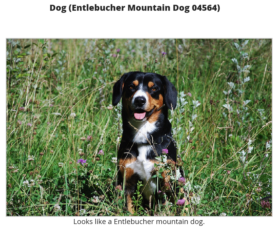
test_two.png

case = "rabbit.jpg"
classifier(case)

test_three.png

Rabbit image from Wikimedia.

case = "hot_dog.jpg"
classifier(case)
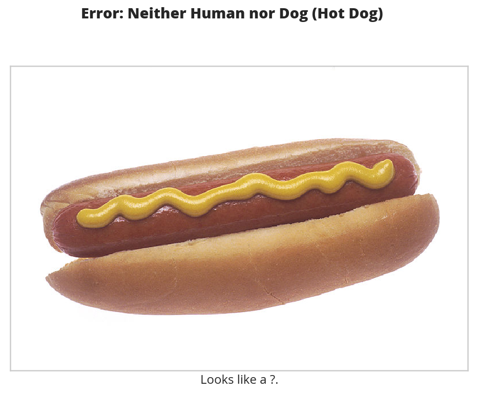
test_four.png

The Hot Dog is also from Wikimedia.

case = human_files_short[34]
classifier(case)

test_five.png

So, somehow my class-based detector got smarter than my function based one and can now tell that this isn't a dog…

MNIST MLP

Introduction

This is from Udacity's Deep Learning Repository which supports their Deep Learning Nanodegree.

We are going to train a Multi-Layer Perceptron to classify images from the MNIST database of hand-written digits.

We're going to do it using the following steps.

  1. Load and visualize the data
  2. Define a neural network
  3. Train the model
  4. Evaluate the performance of our trained model on a test dataset

Imports

From Python

from datetime import datetime

From PyPi

from dotenv import load_dotenv
from torchvision import datasets
import matplotlib.pyplot as pyplot
import seaborn
import torch.nn as nn
import torch.nn.functional as F
import torchvision.transforms as transforms
import torch
import numpy

This Project

from neurotic.tangles.data_paths import DataPathTwo

Setup the Plotting

get_ipython().run_line_magic('matplotlib', 'inline')
seaborn.set(style="whitegrid",
            rc={"axes.grid": False,
                "font.family": ["sans-serif"],
                "font.sans-serif": ["Latin Modern Sans", "Lato"],
                "figure.figsize": (8, 6)},
            font_scale=3)

The Data

The Path To the Data

load_dotenv()
path = DataPathTwo(folder_key="MNIST")
print(path.folder)
print(path.folder.exists())
/home/hades/datasets/MNIST
True

Some Settings

Since I downloaded the data earlier for some other exercise forking sub-processes is probably unnecessary, and for the training and testing we'll use a relatively small batch-size of 20.

WORKERS = 0
BATCH_SIZE = 20

A Transform

We're just going to convert the images to tensors.

transform = transforms.ToTensor()

Split Up the Training and Testing Data

train_data = datasets.MNIST(root=path.folder, train=True,
                            download=True, transform=transform)
test_data = datasets.MNIST(root=path.folder, train=False,
                           download=True, transform=transform)

Create the Batch Loaders

train_batches = torch.utils.data.DataLoader(train_data, batch_size=BATCH_SIZE,
                                            num_workers=WORKERS)
test_batches = torch.utils.data.DataLoader(test_data, batch_size=BATCH_SIZE, 
                                           num_workers=WORKERS)

Visualize a Batch of Training Data

The first step in a classification task is to take a look at the data, make sure it is loaded in correctly, then make any initial observations about patterns in that data.

Grab a batch

images, labels = iter(train_batches).next()
images = images.numpy()

Now that we have a batch we're going to plot the images in the batch, along with the corresponding labels.

figure = pyplot.figure(figsize=(25, 4))
figure.suptitle("First Batch", weight="bold")
for index in numpy.arange(BATCH_SIZE):
    ax = figure.add_subplot(2, BATCH_SIZE/2, index+1, xticks=[], yticks=[])
    ax.imshow(numpy.squeeze(images[index]), cmap='gray')
    # print out the correct label for each image
    # .item() gets the value contained in a Tensor
    ax.set_title(str(labels[index].item()))

batch.png

View a Single Image

Now we're going to take a closer look at the second image in the batch.

image = numpy.squeeze(images[1])

figure = pyplot.figure(figsize = (12,12)) 
ax = figure.add_subplot(111)
ax.imshow(image, cmap='gray')
width, height = image.shape
threshold = image.max()/2.5
for x in range(width):
    for y in range(height):
        val = round(image[x][y],2) if image[x][y] !=0 else 0
        ax.annotate(str(val), xy=(y,x),
                    horizontalalignment='center',
                    verticalalignment='center',
                    color='white' if image[x][y]<threshold else 'black')

image.png

We're looking at a single image with the normalized values for each pixel superimposed on it. It looks like black is 0 and white is 1, although for this image most of the 'white' pixels are just a little less than one.

Define the Network Architecture

The architecture will be responsible for seeing as input a 784-dim Tensor of pixel values for each image, and producing a Tensor of length 10 (our number of classes) that indicates the class scores for an input image. This particular example uses two hidden layers and dropout to avoid overfitting.

These values are based on the keras example implementation.

INPUT_NODES = 28 * 28
HIDDEN_NODES = 512
DROPOUT = 0.2
CLASSES = 10
class Net(nn.Module):
    def __init__(self):
        super().__init__()        
        self.fully_connected_layer_1 = nn.Linear(INPUT_NODES, HIDDEN_NODES)
        self.fully_connected_layer_2 = nn.Linear(HIDDEN_NODES, HIDDEN_NODES)
        self.output = nn.Linear(HIDDEN_NODES, CLASSES)
        self.dropout = nn.Dropout(p=DROPOUT)
        return

    def forward(self, x):
        # flatten image input
        x = x.view(-1, 28 * 28)
        # add hidden layer, with relu activation function
        x = self.dropout(F.relu(self.fully_connected_layer_1(x)))
        x = self.dropout(F.relu(self.fully_connected_layer_2(x)))        
        return self.output(x)

Initialize the NN

model = Net()
print(model)
Net(
  (fully_connected_layer_1): Linear(in_features=784, out_features=512, bias=True)
  (fully_connected_layer_2): Linear(in_features=512, out_features=512, bias=True)
  (output): Linear(in_features=512, out_features=10, bias=True)
  (dropout): Dropout(p=0.2)
)

A Little CUDA

device = torch.device("cuda" if torch.cuda.is_available() else "cpu")
model.to(device)

Specify the Loss Function and Optimizer

It's recommended that you use cross-entropy loss for classification. If you look at the documentation you can see that PyTorch's cross entropy function applies a softmax function to the output layer and then calculates the log loss (so you don't want to do softmax as part of the model output).

criterion = nn.CrossEntropyLoss()
optimizer = torch.optim.SGD(model.parameters(), lr=0.01)

Train the Network

The steps for training/learning from a batch of data are:

  1. Clear the gradients of all optimized variables
  2. Forward pass: compute predicted outputs by passing inputs to the model
  3. Calculate the loss
  4. Backward pass: compute gradient of the loss with respect to model parameters
  5. Perform a single optimization step (parameter update)
  6. Update average training loss

The following loop trains for 30 epochs; feel free to change this number. For now, we suggest somewhere between 20-50 epochs. As you train, take a look at how the values for the training loss decrease over time. We want it to decrease while also avoiding overfitting the training data.

EPOCHS = 30
start = datetime.now()
model.train() # prep model for training

for epoch in range(EPOCHS):
    # monitor training loss
    train_loss = 0.0
    train_losses = []
    # train the model
    for data, target in train_batches:
        # move it to the GPU or CPU
        data, target = data.to(device), target.to(device)
        # clear the gradients of all optimized variables
        optimizer.zero_grad()
        # forward pass: compute predicted outputs by passing inputs to the model
        output = model(data)
        # calculate the loss
        loss = criterion(output, target)
        # backward pass: compute gradient of the loss with respect to model parameters
        loss.backward()
        # perform a single optimization step (parameter update)
        optimizer.step()
        # update running training loss
        train_loss += loss.item() * data.size(0)

        # print training statistics 
        # calculate average loss over an epoch
    train_loss = train_loss/len(train_batches.dataset)
    train_losses.append(train_loss)
    print('Epoch: {} \tTraining Loss: {:.6f}'.format(
        epoch+1, 
        train_loss
        ))
print("Training Time: {}".format(datetime.now() - start))
Epoch: 1        Training Loss: 0.826836
Epoch: 2        Training Loss: 0.324859
Epoch: 3        Training Loss: 0.251608
Epoch: 4        Training Loss: 0.202294
Epoch: 5        Training Loss: 0.170231
Epoch: 6        Training Loss: 0.146775
Epoch: 7        Training Loss: 0.127352
Epoch: 8        Training Loss: 0.115026
Epoch: 9        Training Loss: 0.104332
Epoch: 10       Training Loss: 0.093575
Epoch: 11       Training Loss: 0.084913
Epoch: 12       Training Loss: 0.077826
Epoch: 13       Training Loss: 0.071506
Epoch: 14       Training Loss: 0.067273
Epoch: 15       Training Loss: 0.063749
Epoch: 16       Training Loss: 0.058150
Epoch: 17       Training Loss: 0.054770
Epoch: 18       Training Loss: 0.051584
Epoch: 19       Training Loss: 0.047762
Epoch: 20       Training Loss: 0.045219
Epoch: 21       Training Loss: 0.041732
Epoch: 22       Training Loss: 0.040526
Epoch: 23       Training Loss: 0.038247
Epoch: 24       Training Loss: 0.035713
Epoch: 25       Training Loss: 0.033801
Epoch: 26       Training Loss: 0.031963
Epoch: 27       Training Loss: 0.031082
Epoch: 28       Training Loss: 0.028971
Epoch: 29       Training Loss: 0.027500
Epoch: 30       Training Loss: 0.026876
Training Time: 0:05:59.808071

Test the Trained Network

Finally, we test our best model on previously unseen test data and evaluate it's performance. Testing on unseen data is a good way to check that our model generalizes well. It may also be useful to be granular in this analysis and take a look at how this model performs on each class as well as looking at its overall loss and accuracy.

model.eval()

model.eval() will set all the layers in your model to evaluation mode. This affects layers like dropout layers that turn "off" nodes during training with some probability, but should allow every node to be "on" for evaluation!

Set Up the Testing

test_loss = 0.0
class_correct = list(0. for i in range(10))
class_total = list(0. for i in range(10))
model.eval()

start = datetime.now()

for data, target in test_batches:
    data, target = data.to(device), target.to(device)
    # forward pass: compute predicted outputs by passing inputs to the model
    output = model(data)
    # calculate the loss
    loss = criterion(output, target)
    # update test loss 
    test_loss += loss.item() * data.size(0)
    # convert output probabilities to predicted class
    _, prediction = torch.max(output, 1)
    # compare predictions to true label
    correct = numpy.squeeze(prediction.eq(target.data.view_as(prediction)))
    # calculate test accuracy for each object class
    for i in range(BATCH_SIZE):
        label = target.data[i]
        class_correct[label] += correct[i].item()
        class_total[label] += 1

print("Test Time: {}".format(datetime.now() - start))
Test Time: 0:00:01.860151

Calculate and Print Average Test Loss

test_loss = test_loss/len(test_batches.dataset)
print('Test Loss: {:.6f}\n'.format(test_loss))

for i in range(10):
    if class_total[i] > 0:
        print('Test Accuracy of Batch {}: {:.2f} ({}/{})'.format(
            str(i), 100 * class_correct[i] / class_total[i],
            numpy.sum(class_correct[i]), numpy.sum(class_total[i])))
    else:
        print('Test Accuracy of {}: N/A (no training examples)'.format(classes[i]))

print('\nTest Accuracy (Overall): %2d%% (%2d/%2d)' % (
    100. * numpy.sum(class_correct) / numpy.sum(class_total),
    numpy.sum(class_correct), numpy.sum(class_total)))
Test Loss: 0.056054

Test Accuracy of Batch 0: 99.18 (972.0/980.0)
Test Accuracy of Batch 1: 99.21 (1126.0/1135.0)
Test Accuracy of Batch 2: 98.16 (1013.0/1032.0)
Test Accuracy of Batch 3: 98.02 (990.0/1010.0)
Test Accuracy of Batch 4: 98.47 (967.0/982.0)
Test Accuracy of Batch 5: 98.43 (878.0/892.0)
Test Accuracy of Batch 6: 98.12 (940.0/958.0)
Test Accuracy of Batch 7: 97.47 (1002.0/1028.0)
Test Accuracy of Batch 8: 97.13 (946.0/974.0)
Test Accuracy of Batch 9: 98.12 (990.0/1009.0)

Test Accuracy (Overall): 98% (9824/10000)

Visualize Sample Test Results

This cell displays test images and their labels in this format: predicted (ground-truth). The text will be green for accurately classified examples and red for incorrect predictions.

Obtain One Batch of Test Images

model.cpu()
dataiter = iter(test_batches)
images, labels = dataiter.next()

# get sample outputs
output = model(images)
# convert output probabilities to predicted class
_, preds = torch.max(output, 1)
# prep images for display
images = images.numpy()
# plot the images in the batch, along with predicted and true labels
fig = pyplot.figure(figsize=(25, 4))
for idx in numpy.arange(20):
    ax = fig.add_subplot(2, 20/2, idx+1, xticks=[], yticks=[])
    ax.imshow(numpy.squeeze(images[idx]), cmap='gray')
    ax.set_title("{} ({})".format(str(preds[idx].item()), str(labels[idx].item())),
                 color=("green" if preds[idx]==labels[idx] else "red"))

test.png

This model is surprisingly accurate. I say surprising, even though we created a very accurate model previously, because in my original implementation I used RMSprop as the optimizer, because that's what the Keras implementation used, but then I only got 11%. I'm guessing that there's some extra tuning you need to do to the parameters for RMSprop but I just naively used the defaults. In any case, it semms that SGD is still the champ.

Dog Classification Project Overview

Project Overview

In this project we will build a pipeline that can be used within a web or mobile app to process real-world, user-supplied images. Given an image of a dog, our algorithm will identify an estimate of the canine’s breed. If supplied an image of a human, the code will identify the dog breed that the person most resembles.

The Data

The dog dataset is in a zip-file hosted on Amazon Web Services. The folder should contain three folders (test, train, and valid) and each of these folders should have 133 folders, one for each dog-breed. It looks like the Stanford Dogs Dataset, but the Stanford data set has 120 breeds, so I don't know the actual source. The human dataset seems to be the Labeled Faces in the Wild data set which was built to study the problem of facial recognition. It's made up of real photos of people taken from the web. Each photo sits in a sub-folder that was given the name of the person (e.g. Michelle_Yeoh). The folder hasn't been split into train-test-validiation folders the way the dog dataset was.

Some Rules

  • Unless requested, do not modify code that has already been included.
  • In the notebook, you will need to train CNNs in PyTorch. If your CNN is taking too long to train, feel free to pursue one of the options under the section Accelerating the Training Process below.

(Optionally) Accelerating the Training Process

If your code is taking too long to run, you will need to either reduce the complexity of your chosen CNN architecture or switch to running your code on a GPU. If you'd like to use a GPU, you can spin up an instance of your own:

Amazon Web Services

You can use Amazon Web Services to launch an EC2 GPU instance. (This costs money, but enrolled students should see a coupon code in their student resources.)

Evaluation

Your project will be reviewed by a Udacity reviewer against the CNN project rubric. Review this rubric thoroughly and self-evaluate your project before submission. All criteria found in the rubric must meet specifications for you to pass.

Project Submission

Your submission should consist of the github link to your repository. Your repository should contain:

  • The dog_app.ipynb file with fully functional code, all code cells executed and displaying output, and all questions answered.
  • An HTML or PDF export of the project notebook with the name report.html or report.pdf.

Please do NOT include any of the project data sets provided in the dogImages/ or lfw/ folders.

Transfer Learning One More Time

I spent so much time debugging the original post that I though I'd re-do it without all the flailing around.

Introduction

This is from Udacity's Deep Learning Repository which supports their Deep Learning Nanodegree.

This uses a model trained on ImageNet (available from torchvision) to classify the dataset of cat and dog photos that we used earlier. We're going to use a method called transfer learning where we will use the layers of the pretrained model all the way up until the final classifier which we will define ourselves and train on our new data-set. This way we can take advantage of what the model has already learned for image detection and only train a few layers.

Set Up

Imports

Python

from collections import OrderedDict
from datetime import datetime

PyPi

from torch import nn
from torch import optim
from torchvision import datasets, transforms, models
import torch
import torch.nn.functional as F

This Project

from neurotic.tangles.data_paths import DataPathTwo
from neurotic.models.fashion import (
    train_only,
    test_only,
    )

Dotenv

For some reason dotenv has stopped working unless it's called in the notebook. Maybe this will fix it

The Data

We're going to have to resize the images to be 224x224 to work with the pre-trained models and match the means ([0.485, 0.456, 0.406]) and the standard deviations ([0.229, 0.224, 0.225]) that were used to normalize the original data set.

means = [0.485, 0.456, 0.406]
deviations = [0.229, 0.224, 0.225]
PIXELS = 224

train_transforms = transforms.Compose([transforms.RandomRotation(30),
                                       transforms.RandomResizedCrop(PIXELS),
                                       transforms.RandomHorizontalFlip(),
                                       transforms.ToTensor(),
                                       transforms.Normalize(means,
                                                            deviations)])

test_transforms = transforms.Compose([transforms.Resize(255),
                                      transforms.CenterCrop(PIXELS),
                                      transforms.ToTensor(),
                                      transforms.Normalize(means,
                                                           deviations)])

Load the Data

As I mentioned we're using the same Cat and Dog images as before. So first I make my path-setter (which maybe isn't as useful as it was when I had dotenv working better).

train_path = DataPathTwo(folder_key="CAT_DOG_TRAIN")
test_path = DataPathTwo(folder_key="CAT_DOG_TEST")

So now we set up the testing and training data sets.

train_data = datasets.ImageFolder(train_path.folder,
                                  transform=train_transforms)
test_data = datasets.ImageFolder(test_path.folder,
                                 transform=test_transforms)

And create the batch-iterators with a batch-size of 64.

BATCH_SIZE = 64
train_batches = torch.utils.data.DataLoader(train_data, batch_size=BATCH_SIZE,
                                            shuffle=True)
test_batches = torch.utils.data.DataLoader(test_data, batch_size=BATCH_SIZE)

The DenseNet Model

I'm going to load the DenseNet model.

model = models.densenet121(pretrained=True)

It actually emits a warning that the code is using an incorrect method call somewhere, but I'll ignore that.

UserWarning: nn.init.kaiming_normal is now deprecated in favor of nn.init.kaiming_normal_.
 nn.init.kaiming_normal(m.weight.data)

Freeze The Model Parameters

We need to freeze the parameters before training so we don't end up trying to re-train our pre-trained network.

for param in model.parameters():
    param.requires_grad = False

The Classifier

So this is the part where we add our own classifier at the end so that we can train it on cats and dogs. I'll use the original 500 fully connected nodes instead of the 256 I ended up with in my previous attempt.

To figure out the inputs to the layer we can just look at the original classifier layer in the model.

print(model.classifier)
Linear(in_features=1024, out_features=1000, bias=True)

So we need to make sure we have 1,024 inputs to our classification layer and change the number of outputs to 2 (since we have only dogs and cats). We're also going to use two layers, the first one will have a ReLU activation and the second (the output) will have a Log-Softmax activation.

HIDDEN_NODES = 500
INPUT_NODES = 1024
OUTPUT_NODES = 2
classifier = nn.Sequential(OrderedDict([
                          ('fully_connected_layer',
                           nn.Linear(INPUT_NODES, HIDDEN_NODES)),
                          ('relu', nn.ReLU()),
                          ("dropout", nn.Dropout(p=0.2)),
                          ('fully_connected_layer_2',
                           nn.Linear(HIDDEN_NODES, OUTPUT_NODES)),
                          ('output', nn.LogSoftmax(dim=1))
                          ]))
model.classifier = classifier

So we now have a (mostly) pre-trained deep neural network with an untrained classifier.

Add Some CUDA

To speed this up somewhat I'll add (if it's available) a little cuda.

device = torch.device("cuda" if torch.cuda.is_available() else "cpu")
model.to(device)

Add some more CUDA

This next bit doesn't work on any of my machines, but maybe someday.

if torch.cuda.device_count() > 1:
    print("Using {} GPUs".format(torch.cuda.device_count()))
    model = nn.DataParallel(model)
    model.to(device)
else:
    print("Only 1 GPU available")
Only 1 GPU available

Train It

First we'll set up our criterion - Negative Log Likelihood Loss (NLLLoss) and optimizer - Adam Optimization. Amazingly this only needs one pass through the data set. There's 352 batches in the training data-set so I won't print out each of the outcomes for the epochs.

LEARNING_RATE = 0.003
EPOCHS = 1
criterion = nn.NLLLoss()
optimizer = optim.Adam(model.classifier.parameters(), lr=LEARNING_RATE)
start = datetime.now()
outcome = train_only(model, optimizer, criterion,
                     train_batches,
                     epochs=EPOCHS, emit=False, device=device)
print("Training Time: {}".format(datetime.now() - start))
Training Time: 0:10:35.847469
start = datetime.now()
test_outcome = test_only(model, test_batches, device)
print("Test Time: {}".format(datetime.now() - start))
Test Time: 0:00:46.695136
print(test_outcome)
0.9788

The key bit here was that I was earlier forgetting to add dropout, dropping the accuracy to between .5 and .6.

Tips, Tricks and Other Notes

On Shapes

As the tensors go through the model you should check the shapes to make sure they are correct (or at least what you expect).

Troubleshooting Training

  • Make sure you are clearing the gradients in the training loop with optimizer.zero_grad()
  • In the validation loop, set the network to evaluation mode with model.eval() and then back to training mode with model.train

CUDA Problems

If you see an error saying pytorch Expected an object of type torch.FloatTensor but found type torch.cuda.FloatTensor then it means something is trying to be run on the CPU but something else wants to use the GPU. Make sure you called .to(device) on the model and all your tensors (including the data).

Part 8 - Transfer Learning

Introduction

This is from Udacity's Deep Learning Repository which supports their Deep Learning Nanodegree.

In this notebook, you'll learn how to use pre-trained networks to solved challenging problems in computer vision. Specifically, you'll use networks trained on ImageNet (available from torchvision).

ImageNet is a massive dataset with over 1 million labeled images in 1000 categories. It's used to train deep neural networks using an architecture called convolutional layers. I'm not going to get into the details of convolutional networks here, but if you want to learn more about them, please watch this.

Once trained, these models work astonishingly well as feature detectors for images they weren't trained on. Using a pre-trained network on images not in the training set is called transfer learning. Here we'll use transfer learning to train a network that can classify our cat and dog photos with near perfect accuracy.

With torchvision.models you can download these pre-trained networks and use them in your applications. We'll include models in our imports now.

Set Up

Imports

Python

from collections import OrderedDict
from datetime import datetime

PyPi

from torch import nn
from torch import optim
from torchvision import datasets, transforms, models
import torch
import torch.nn.functional as F

This Project

from neurotic.tangles.data_paths import DataPathTwo
from neurotic.models.fashion import (
    test_only,
    train_only,
    )

Dotenv

For some reason dotenv has stopped working unless it's called in the notebook. Maybe this will fix it

The Data

Most of the pretrained models require the input to be 224x224 images. Also, we'll need to match the normalization used when the models were trained. Each color channel was normalized separately, the means are [0.485, 0.456, 0.406] and the standard deviations are [0.229, 0.224, 0.225].

means = [0.485, 0.456, 0.406]
deviations = [0.229, 0.224, 0.225]

train_transforms = transforms.Compose([transforms.RandomRotation(30),
                                       transforms.RandomResizedCrop(224),
                                       transforms.RandomHorizontalFlip(),
                                       transforms.ToTensor(),
                                       transforms.Normalize(means,
                                                            deviations)])

test_transforms = transforms.Compose([transforms.Resize(255),
                                      transforms.CenterCrop(224),
                                      transforms.ToTensor(),
                                      transforms.Normalize(means,
                                                           deviations)])

Load the Data

We're going to load the Cat-Dog data set again.

train_path = DataPathTwo(folder_key="CAT_DOG_TRAIN")
test_path = DataPathTwo(folder_key="CAT_DOG_TEST")
train_data = datasets.ImageFolder(train_path.folder, transform=train_transforms)
test_data = datasets.ImageFolder(test_path.folder, transform=test_transforms)
train_batches = torch.utils.data.DataLoader(train_data, batch_size=64,
                                            shuffle=True)
test_batches = torch.utils.data.DataLoader(test_data, batch_size=64)

The DenseNet Model

We are going to load the DenseNet model.

model = models.densenet121(pretrained=True)
print(model)
DenseNet(
  (features): Sequential(
    (conv0): Conv2d(3, 64, kernel_size=(7, 7), stride=(2, 2), padding=(3, 3), bias=False)
    (norm0): BatchNorm2d(64, eps=1e-05, momentum=0.1, affine=True, track_running_stats=True)
    (relu0): ReLU(inplace)
    (pool0): MaxPool2d(kernel_size=3, stride=2, padding=1, dilation=1, ceil_mode=False)
    (denseblock1): _DenseBlock(
      (denselayer1): _DenseLayer(
        (norm1): BatchNorm2d(64, eps=1e-05, momentum=0.1, affine=True, track_running_stats=True)
        (relu1): ReLU(inplace)
        (conv1): Conv2d(64, 128, kernel_size=(1, 1), stride=(1, 1), bias=False)
        (norm2): BatchNorm2d(128, eps=1e-05, momentum=0.1, affine=True, track_running_stats=True)
        (relu2): ReLU(inplace)
        (conv2): Conv2d(128, 32, kernel_size=(3, 3), stride=(1, 1), padding=(1, 1), bias=False)
      )
      (denselayer2): _DenseLayer(
        (norm1): BatchNorm2d(96, eps=1e-05, momentum=0.1, affine=True, track_running_stats=True)
        (relu1): ReLU(inplace)
        (conv1): Conv2d(96, 128, kernel_size=(1, 1), stride=(1, 1), bias=False)
        (norm2): BatchNorm2d(128, eps=1e-05, momentum=0.1, affine=True, track_running_stats=True)
        (relu2): ReLU(inplace)
        (conv2): Conv2d(128, 32, kernel_size=(3, 3), stride=(1, 1), padding=(1, 1), bias=False)
      )
      (denselayer3): _DenseLayer(
        (norm1): BatchNorm2d(128, eps=1e-05, momentum=0.1, affine=True, track_running_stats=True)
        (relu1): ReLU(inplace)
        (conv1): Conv2d(128, 128, kernel_size=(1, 1), stride=(1, 1), bias=False)
        (norm2): BatchNorm2d(128, eps=1e-05, momentum=0.1, affine=True, track_running_stats=True)
        (relu2): ReLU(inplace)
        (conv2): Conv2d(128, 32, kernel_size=(3, 3), stride=(1, 1), padding=(1, 1), bias=False)
      )
      (denselayer4): _DenseLayer(
        (norm1): BatchNorm2d(160, eps=1e-05, momentum=0.1, affine=True, track_running_stats=True)
        (relu1): ReLU(inplace)
        (conv1): Conv2d(160, 128, kernel_size=(1, 1), stride=(1, 1), bias=False)
        (norm2): BatchNorm2d(128, eps=1e-05, momentum=0.1, affine=True, track_running_stats=True)
        (relu2): ReLU(inplace)
        (conv2): Conv2d(128, 32, kernel_size=(3, 3), stride=(1, 1), padding=(1, 1), bias=False)
      )
      (denselayer5): _DenseLayer(
        (norm1): BatchNorm2d(192, eps=1e-05, momentum=0.1, affine=True, track_running_stats=True)
        (relu1): ReLU(inplace)
        (conv1): Conv2d(192, 128, kernel_size=(1, 1), stride=(1, 1), bias=False)
        (norm2): BatchNorm2d(128, eps=1e-05, momentum=0.1, affine=True, track_running_stats=True)
        (relu2): ReLU(inplace)
        (conv2): Conv2d(128, 32, kernel_size=(3, 3), stride=(1, 1), padding=(1, 1), bias=False)
      )
      (denselayer6): _DenseLayer(
        (norm1): BatchNorm2d(224, eps=1e-05, momentum=0.1, affine=True, track_running_stats=True)
        (relu1): ReLU(inplace)
        (conv1): Conv2d(224, 128, kernel_size=(1, 1), stride=(1, 1), bias=False)
        (norm2): BatchNorm2d(128, eps=1e-05, momentum=0.1, affine=True, track_running_stats=True)
        (relu2): ReLU(inplace)
        (conv2): Conv2d(128, 32, kernel_size=(3, 3), stride=(1, 1), padding=(1, 1), bias=False)
      )
    )
    (transition1): _Transition(
      (norm): BatchNorm2d(256, eps=1e-05, momentum=0.1, affine=True, track_running_stats=True)
      (relu): ReLU(inplace)
      (conv): Conv2d(256, 128, kernel_size=(1, 1), stride=(1, 1), bias=False)
      (pool): AvgPool2d(kernel_size=2, stride=2, padding=0)
    )
    (denseblock2): _DenseBlock(
      (denselayer1): _DenseLayer(
        (norm1): BatchNorm2d(128, eps=1e-05, momentum=0.1, affine=True, track_running_stats=True)
        (relu1): ReLU(inplace)
        (conv1): Conv2d(128, 128, kernel_size=(1, 1), stride=(1, 1), bias=False)
        (norm2): BatchNorm2d(128, eps=1e-05, momentum=0.1, affine=True, track_running_stats=True)
        (relu2): ReLU(inplace)
        (conv2): Conv2d(128, 32, kernel_size=(3, 3), stride=(1, 1), padding=(1, 1), bias=False)
      )
      (denselayer2): _DenseLayer(
        (norm1): BatchNorm2d(160, eps=1e-05, momentum=0.1, affine=True, track_running_stats=True)
        (relu1): ReLU(inplace)
        (conv1): Conv2d(160, 128, kernel_size=(1, 1), stride=(1, 1), bias=False)
        (norm2): BatchNorm2d(128, eps=1e-05, momentum=0.1, affine=True, track_running_stats=True)
        (relu2): ReLU(inplace)
        (conv2): Conv2d(128, 32, kernel_size=(3, 3), stride=(1, 1), padding=(1, 1), bias=False)
      )
      (denselayer3): _DenseLayer(
        (norm1): BatchNorm2d(192, eps=1e-05, momentum=0.1, affine=True, track_running_stats=True)
        (relu1): ReLU(inplace)
        (conv1): Conv2d(192, 128, kernel_size=(1, 1), stride=(1, 1), bias=False)
        (norm2): BatchNorm2d(128, eps=1e-05, momentum=0.1, affine=True, track_running_stats=True)
        (relu2): ReLU(inplace)
        (conv2): Conv2d(128, 32, kernel_size=(3, 3), stride=(1, 1), padding=(1, 1), bias=False)
      )
      (denselayer4): _DenseLayer(
        (norm1): BatchNorm2d(224, eps=1e-05, momentum=0.1, affine=True, track_running_stats=True)
        (relu1): ReLU(inplace)
        (conv1): Conv2d(224, 128, kernel_size=(1, 1), stride=(1, 1), bias=False)
        (norm2): BatchNorm2d(128, eps=1e-05, momentum=0.1, affine=True, track_running_stats=True)
        (relu2): ReLU(inplace)
        (conv2): Conv2d(128, 32, kernel_size=(3, 3), stride=(1, 1), padding=(1, 1), bias=False)
      )
      (denselayer5): _DenseLayer(
        (norm1): BatchNorm2d(256, eps=1e-05, momentum=0.1, affine=True, track_running_stats=True)
        (relu1): ReLU(inplace)
        (conv1): Conv2d(256, 128, kernel_size=(1, 1), stride=(1, 1), bias=False)
        (norm2): BatchNorm2d(128, eps=1e-05, momentum=0.1, affine=True, track_running_stats=True)
        (relu2): ReLU(inplace)
        (conv2): Conv2d(128, 32, kernel_size=(3, 3), stride=(1, 1), padding=(1, 1), bias=False)
      )
      (denselayer6): _DenseLayer(
        (norm1): BatchNorm2d(288, eps=1e-05, momentum=0.1, affine=True, track_running_stats=True)
        (relu1): ReLU(inplace)
        (conv1): Conv2d(288, 128, kernel_size=(1, 1), stride=(1, 1), bias=False)
        (norm2): BatchNorm2d(128, eps=1e-05, momentum=0.1, affine=True, track_running_stats=True)
        (relu2): ReLU(inplace)
        (conv2): Conv2d(128, 32, kernel_size=(3, 3), stride=(1, 1), padding=(1, 1), bias=False)
      )
      (denselayer7): _DenseLayer(
        (norm1): BatchNorm2d(320, eps=1e-05, momentum=0.1, affine=True, track_running_stats=True)
        (relu1): ReLU(inplace)
        (conv1): Conv2d(320, 128, kernel_size=(1, 1), stride=(1, 1), bias=False)
        (norm2): BatchNorm2d(128, eps=1e-05, momentum=0.1, affine=True, track_running_stats=True)
        (relu2): ReLU(inplace)
        (conv2): Conv2d(128, 32, kernel_size=(3, 3), stride=(1, 1), padding=(1, 1), bias=False)
      )
      (denselayer8): _DenseLayer(
        (norm1): BatchNorm2d(352, eps=1e-05, momentum=0.1, affine=True, track_running_stats=True)
        (relu1): ReLU(inplace)
        (conv1): Conv2d(352, 128, kernel_size=(1, 1), stride=(1, 1), bias=False)
        (norm2): BatchNorm2d(128, eps=1e-05, momentum=0.1, affine=True, track_running_stats=True)
        (relu2): ReLU(inplace)
        (conv2): Conv2d(128, 32, kernel_size=(3, 3), stride=(1, 1), padding=(1, 1), bias=False)
      )
      (denselayer9): _DenseLayer(
        (norm1): BatchNorm2d(384, eps=1e-05, momentum=0.1, affine=True, track_running_stats=True)
        (relu1): ReLU(inplace)
        (conv1): Conv2d(384, 128, kernel_size=(1, 1), stride=(1, 1), bias=False)
        (norm2): BatchNorm2d(128, eps=1e-05, momentum=0.1, affine=True, track_running_stats=True)
        (relu2): ReLU(inplace)
        (conv2): Conv2d(128, 32, kernel_size=(3, 3), stride=(1, 1), padding=(1, 1), bias=False)
      )
      (denselayer10): _DenseLayer(
        (norm1): BatchNorm2d(416, eps=1e-05, momentum=0.1, affine=True, track_running_stats=True)
        (relu1): ReLU(inplace)
        (conv1): Conv2d(416, 128, kernel_size=(1, 1), stride=(1, 1), bias=False)
        (norm2): BatchNorm2d(128, eps=1e-05, momentum=0.1, affine=True, track_running_stats=True)
        (relu2): ReLU(inplace)
        (conv2): Conv2d(128, 32, kernel_size=(3, 3), stride=(1, 1), padding=(1, 1), bias=False)
      )
      (denselayer11): _DenseLayer(
        (norm1): BatchNorm2d(448, eps=1e-05, momentum=0.1, affine=True, track_running_stats=True)
        (relu1): ReLU(inplace)
        (conv1): Conv2d(448, 128, kernel_size=(1, 1), stride=(1, 1), bias=False)
        (norm2): BatchNorm2d(128, eps=1e-05, momentum=0.1, affine=True, track_running_stats=True)
        (relu2): ReLU(inplace)
        (conv2): Conv2d(128, 32, kernel_size=(3, 3), stride=(1, 1), padding=(1, 1), bias=False)
      )
      (denselayer12): _DenseLayer(
        (norm1): BatchNorm2d(480, eps=1e-05, momentum=0.1, affine=True, track_running_stats=True)
        (relu1): ReLU(inplace)
        (conv1): Conv2d(480, 128, kernel_size=(1, 1), stride=(1, 1), bias=False)
        (norm2): BatchNorm2d(128, eps=1e-05, momentum=0.1, affine=True, track_running_stats=True)
        (relu2): ReLU(inplace)
        (conv2): Conv2d(128, 32, kernel_size=(3, 3), stride=(1, 1), padding=(1, 1), bias=False)
      )
    )
    (transition2): _Transition(
      (norm): BatchNorm2d(512, eps=1e-05, momentum=0.1, affine=True, track_running_stats=True)
      (relu): ReLU(inplace)
      (conv): Conv2d(512, 256, kernel_size=(1, 1), stride=(1, 1), bias=False)
      (pool): AvgPool2d(kernel_size=2, stride=2, padding=0)
    )
    (denseblock3): _DenseBlock(
      (denselayer1): _DenseLayer(
        (norm1): BatchNorm2d(256, eps=1e-05, momentum=0.1, affine=True, track_running_stats=True)
        (relu1): ReLU(inplace)
        (conv1): Conv2d(256, 128, kernel_size=(1, 1), stride=(1, 1), bias=False)
        (norm2): BatchNorm2d(128, eps=1e-05, momentum=0.1, affine=True, track_running_stats=True)
        (relu2): ReLU(inplace)
        (conv2): Conv2d(128, 32, kernel_size=(3, 3), stride=(1, 1), padding=(1, 1), bias=False)
      )
      (denselayer2): _DenseLayer(
        (norm1): BatchNorm2d(288, eps=1e-05, momentum=0.1, affine=True, track_running_stats=True)
        (relu1): ReLU(inplace)
        (conv1): Conv2d(288, 128, kernel_size=(1, 1), stride=(1, 1), bias=False)
        (norm2): BatchNorm2d(128, eps=1e-05, momentum=0.1, affine=True, track_running_stats=True)
        (relu2): ReLU(inplace)
        (conv2): Conv2d(128, 32, kernel_size=(3, 3), stride=(1, 1), padding=(1, 1), bias=False)
      )
      (denselayer3): _DenseLayer(
        (norm1): BatchNorm2d(320, eps=1e-05, momentum=0.1, affine=True, track_running_stats=True)
        (relu1): ReLU(inplace)
        (conv1): Conv2d(320, 128, kernel_size=(1, 1), stride=(1, 1), bias=False)
        (norm2): BatchNorm2d(128, eps=1e-05, momentum=0.1, affine=True, track_running_stats=True)
        (relu2): ReLU(inplace)
        (conv2): Conv2d(128, 32, kernel_size=(3, 3), stride=(1, 1), padding=(1, 1), bias=False)
      )
      (denselayer4): _DenseLayer(
        (norm1): BatchNorm2d(352, eps=1e-05, momentum=0.1, affine=True, track_running_stats=True)
        (relu1): ReLU(inplace)
        (conv1): Conv2d(352, 128, kernel_size=(1, 1), stride=(1, 1), bias=False)
        (norm2): BatchNorm2d(128, eps=1e-05, momentum=0.1, affine=True, track_running_stats=True)
        (relu2): ReLU(inplace)
        (conv2): Conv2d(128, 32, kernel_size=(3, 3), stride=(1, 1), padding=(1, 1), bias=False)
      )
      (denselayer5): _DenseLayer(
        (norm1): BatchNorm2d(384, eps=1e-05, momentum=0.1, affine=True, track_running_stats=True)
        (relu1): ReLU(inplace)
        (conv1): Conv2d(384, 128, kernel_size=(1, 1), stride=(1, 1), bias=False)
        (norm2): BatchNorm2d(128, eps=1e-05, momentum=0.1, affine=True, track_running_stats=True)
        (relu2): ReLU(inplace)
        (conv2): Conv2d(128, 32, kernel_size=(3, 3), stride=(1, 1), padding=(1, 1), bias=False)
      )
      (denselayer6): _DenseLayer(
        (norm1): BatchNorm2d(416, eps=1e-05, momentum=0.1, affine=True, track_running_stats=True)
        (relu1): ReLU(inplace)
        (conv1): Conv2d(416, 128, kernel_size=(1, 1), stride=(1, 1), bias=False)
        (norm2): BatchNorm2d(128, eps=1e-05, momentum=0.1, affine=True, track_running_stats=True)
        (relu2): ReLU(inplace)
        (conv2): Conv2d(128, 32, kernel_size=(3, 3), stride=(1, 1), padding=(1, 1), bias=False)
      )
      (denselayer7): _DenseLayer(
        (norm1): BatchNorm2d(448, eps=1e-05, momentum=0.1, affine=True, track_running_stats=True)
        (relu1): ReLU(inplace)
        (conv1): Conv2d(448, 128, kernel_size=(1, 1), stride=(1, 1), bias=False)
        (norm2): BatchNorm2d(128, eps=1e-05, momentum=0.1, affine=True, track_running_stats=True)
        (relu2): ReLU(inplace)
        (conv2): Conv2d(128, 32, kernel_size=(3, 3), stride=(1, 1), padding=(1, 1), bias=False)
      )
      (denselayer8): _DenseLayer(
        (norm1): BatchNorm2d(480, eps=1e-05, momentum=0.1, affine=True, track_running_stats=True)
        (relu1): ReLU(inplace)
        (conv1): Conv2d(480, 128, kernel_size=(1, 1), stride=(1, 1), bias=False)
        (norm2): BatchNorm2d(128, eps=1e-05, momentum=0.1, affine=True, track_running_stats=True)
        (relu2): ReLU(inplace)
        (conv2): Conv2d(128, 32, kernel_size=(3, 3), stride=(1, 1), padding=(1, 1), bias=False)
      )
      (denselayer9): _DenseLayer(
        (norm1): BatchNorm2d(512, eps=1e-05, momentum=0.1, affine=True, track_running_stats=True)
        (relu1): ReLU(inplace)
        (conv1): Conv2d(512, 128, kernel_size=(1, 1), stride=(1, 1), bias=False)
        (norm2): BatchNorm2d(128, eps=1e-05, momentum=0.1, affine=True, track_running_stats=True)
        (relu2): ReLU(inplace)
        (conv2): Conv2d(128, 32, kernel_size=(3, 3), stride=(1, 1), padding=(1, 1), bias=False)
      )
      (denselayer10): _DenseLayer(
        (norm1): BatchNorm2d(544, eps=1e-05, momentum=0.1, affine=True, track_running_stats=True)
        (relu1): ReLU(inplace)
        (conv1): Conv2d(544, 128, kernel_size=(1, 1), stride=(1, 1), bias=False)
        (norm2): BatchNorm2d(128, eps=1e-05, momentum=0.1, affine=True, track_running_stats=True)
        (relu2): ReLU(inplace)
        (conv2): Conv2d(128, 32, kernel_size=(3, 3), stride=(1, 1), padding=(1, 1), bias=False)
      )
      (denselayer11): _DenseLayer(
        (norm1): BatchNorm2d(576, eps=1e-05, momentum=0.1, affine=True, track_running_stats=True)
        (relu1): ReLU(inplace)
        (conv1): Conv2d(576, 128, kernel_size=(1, 1), stride=(1, 1), bias=False)
        (norm2): BatchNorm2d(128, eps=1e-05, momentum=0.1, affine=True, track_running_stats=True)
        (relu2): ReLU(inplace)
        (conv2): Conv2d(128, 32, kernel_size=(3, 3), stride=(1, 1), padding=(1, 1), bias=False)
      )
      (denselayer12): _DenseLayer(
        (norm1): BatchNorm2d(608, eps=1e-05, momentum=0.1, affine=True, track_running_stats=True)
        (relu1): ReLU(inplace)
        (conv1): Conv2d(608, 128, kernel_size=(1, 1), stride=(1, 1), bias=False)
        (norm2): BatchNorm2d(128, eps=1e-05, momentum=0.1, affine=True, track_running_stats=True)
        (relu2): ReLU(inplace)
        (conv2): Conv2d(128, 32, kernel_size=(3, 3), stride=(1, 1), padding=(1, 1), bias=False)
      )
      (denselayer13): _DenseLayer(
        (norm1): BatchNorm2d(640, eps=1e-05, momentum=0.1, affine=True, track_running_stats=True)
        (relu1): ReLU(inplace)
        (conv1): Conv2d(640, 128, kernel_size=(1, 1), stride=(1, 1), bias=False)
        (norm2): BatchNorm2d(128, eps=1e-05, momentum=0.1, affine=True, track_running_stats=True)
        (relu2): ReLU(inplace)
        (conv2): Conv2d(128, 32, kernel_size=(3, 3), stride=(1, 1), padding=(1, 1), bias=False)
      )
      (denselayer14): _DenseLayer(
        (norm1): BatchNorm2d(672, eps=1e-05, momentum=0.1, affine=True, track_running_stats=True)
        (relu1): ReLU(inplace)
        (conv1): Conv2d(672, 128, kernel_size=(1, 1), stride=(1, 1), bias=False)
        (norm2): BatchNorm2d(128, eps=1e-05, momentum=0.1, affine=True, track_running_stats=True)
        (relu2): ReLU(inplace)
        (conv2): Conv2d(128, 32, kernel_size=(3, 3), stride=(1, 1), padding=(1, 1), bias=False)
      )
      (denselayer15): _DenseLayer(
        (norm1): BatchNorm2d(704, eps=1e-05, momentum=0.1, affine=True, track_running_stats=True)
        (relu1): ReLU(inplace)
        (conv1): Conv2d(704, 128, kernel_size=(1, 1), stride=(1, 1), bias=False)
        (norm2): BatchNorm2d(128, eps=1e-05, momentum=0.1, affine=True, track_running_stats=True)
        (relu2): ReLU(inplace)
        (conv2): Conv2d(128, 32, kernel_size=(3, 3), stride=(1, 1), padding=(1, 1), bias=False)
      )
      (denselayer16): _DenseLayer(
        (norm1): BatchNorm2d(736, eps=1e-05, momentum=0.1, affine=True, track_running_stats=True)
        (relu1): ReLU(inplace)
        (conv1): Conv2d(736, 128, kernel_size=(1, 1), stride=(1, 1), bias=False)
        (norm2): BatchNorm2d(128, eps=1e-05, momentum=0.1, affine=True, track_running_stats=True)
        (relu2): ReLU(inplace)
        (conv2): Conv2d(128, 32, kernel_size=(3, 3), stride=(1, 1), padding=(1, 1), bias=False)
      )
      (denselayer17): _DenseLayer(
        (norm1): BatchNorm2d(768, eps=1e-05, momentum=0.1, affine=True, track_running_stats=True)
        (relu1): ReLU(inplace)
        (conv1): Conv2d(768, 128, kernel_size=(1, 1), stride=(1, 1), bias=False)
        (norm2): BatchNorm2d(128, eps=1e-05, momentum=0.1, affine=True, track_running_stats=True)
        (relu2): ReLU(inplace)
        (conv2): Conv2d(128, 32, kernel_size=(3, 3), stride=(1, 1), padding=(1, 1), bias=False)
      )
      (denselayer18): _DenseLayer(
        (norm1): BatchNorm2d(800, eps=1e-05, momentum=0.1, affine=True, track_running_stats=True)
        (relu1): ReLU(inplace)
        (conv1): Conv2d(800, 128, kernel_size=(1, 1), stride=(1, 1), bias=False)
        (norm2): BatchNorm2d(128, eps=1e-05, momentum=0.1, affine=True, track_running_stats=True)
        (relu2): ReLU(inplace)
        (conv2): Conv2d(128, 32, kernel_size=(3, 3), stride=(1, 1), padding=(1, 1), bias=False)
      )
      (denselayer19): _DenseLayer(
        (norm1): BatchNorm2d(832, eps=1e-05, momentum=0.1, affine=True, track_running_stats=True)
        (relu1): ReLU(inplace)
        (conv1): Conv2d(832, 128, kernel_size=(1, 1), stride=(1, 1), bias=False)
        (norm2): BatchNorm2d(128, eps=1e-05, momentum=0.1, affine=True, track_running_stats=True)
        (relu2): ReLU(inplace)
        (conv2): Conv2d(128, 32, kernel_size=(3, 3), stride=(1, 1), padding=(1, 1), bias=False)
      )
      (denselayer20): _DenseLayer(
        (norm1): BatchNorm2d(864, eps=1e-05, momentum=0.1, affine=True, track_running_stats=True)
        (relu1): ReLU(inplace)
        (conv1): Conv2d(864, 128, kernel_size=(1, 1), stride=(1, 1), bias=False)
        (norm2): BatchNorm2d(128, eps=1e-05, momentum=0.1, affine=True, track_running_stats=True)
        (relu2): ReLU(inplace)
        (conv2): Conv2d(128, 32, kernel_size=(3, 3), stride=(1, 1), padding=(1, 1), bias=False)
      )
      (denselayer21): _DenseLayer(
        (norm1): BatchNorm2d(896, eps=1e-05, momentum=0.1, affine=True, track_running_stats=True)
        (relu1): ReLU(inplace)
        (conv1): Conv2d(896, 128, kernel_size=(1, 1), stride=(1, 1), bias=False)
        (norm2): BatchNorm2d(128, eps=1e-05, momentum=0.1, affine=True, track_running_stats=True)
        (relu2): ReLU(inplace)
        (conv2): Conv2d(128, 32, kernel_size=(3, 3), stride=(1, 1), padding=(1, 1), bias=False)
      )
      (denselayer22): _DenseLayer(
        (norm1): BatchNorm2d(928, eps=1e-05, momentum=0.1, affine=True, track_running_stats=True)
        (relu1): ReLU(inplace)
        (conv1): Conv2d(928, 128, kernel_size=(1, 1), stride=(1, 1), bias=False)
        (norm2): BatchNorm2d(128, eps=1e-05, momentum=0.1, affine=True, track_running_stats=True)
        (relu2): ReLU(inplace)
        (conv2): Conv2d(128, 32, kernel_size=(3, 3), stride=(1, 1), padding=(1, 1), bias=False)
      )
      (denselayer23): _DenseLayer(
        (norm1): BatchNorm2d(960, eps=1e-05, momentum=0.1, affine=True, track_running_stats=True)
        (relu1): ReLU(inplace)
        (conv1): Conv2d(960, 128, kernel_size=(1, 1), stride=(1, 1), bias=False)
        (norm2): BatchNorm2d(128, eps=1e-05, momentum=0.1, affine=True, track_running_stats=True)
        (relu2): ReLU(inplace)
        (conv2): Conv2d(128, 32, kernel_size=(3, 3), stride=(1, 1), padding=(1, 1), bias=False)
      )
      (denselayer24): _DenseLayer(
        (norm1): BatchNorm2d(992, eps=1e-05, momentum=0.1, affine=True, track_running_stats=True)
        (relu1): ReLU(inplace)
        (conv1): Conv2d(992, 128, kernel_size=(1, 1), stride=(1, 1), bias=False)
        (norm2): BatchNorm2d(128, eps=1e-05, momentum=0.1, affine=True, track_running_stats=True)
        (relu2): ReLU(inplace)
        (conv2): Conv2d(128, 32, kernel_size=(3, 3), stride=(1, 1), padding=(1, 1), bias=False)
      )
    )
    (transition3): _Transition(
      (norm): BatchNorm2d(1024, eps=1e-05, momentum=0.1, affine=True, track_running_stats=True)
      (relu): ReLU(inplace)
      (conv): Conv2d(1024, 512, kernel_size=(1, 1), stride=(1, 1), bias=False)
      (pool): AvgPool2d(kernel_size=2, stride=2, padding=0)
    )
    (denseblock4): _DenseBlock(
      (denselayer1): _DenseLayer(
        (norm1): BatchNorm2d(512, eps=1e-05, momentum=0.1, affine=True, track_running_stats=True)
        (relu1): ReLU(inplace)
        (conv1): Conv2d(512, 128, kernel_size=(1, 1), stride=(1, 1), bias=False)
        (norm2): BatchNorm2d(128, eps=1e-05, momentum=0.1, affine=True, track_running_stats=True)
        (relu2): ReLU(inplace)
        (conv2): Conv2d(128, 32, kernel_size=(3, 3), stride=(1, 1), padding=(1, 1), bias=False)
      )
      (denselayer2): _DenseLayer(
        (norm1): BatchNorm2d(544, eps=1e-05, momentum=0.1, affine=True, track_running_stats=True)
        (relu1): ReLU(inplace)
        (conv1): Conv2d(544, 128, kernel_size=(1, 1), stride=(1, 1), bias=False)
        (norm2): BatchNorm2d(128, eps=1e-05, momentum=0.1, affine=True, track_running_stats=True)
        (relu2): ReLU(inplace)
        (conv2): Conv2d(128, 32, kernel_size=(3, 3), stride=(1, 1), padding=(1, 1), bias=False)
      )
      (denselayer3): _DenseLayer(
        (norm1): BatchNorm2d(576, eps=1e-05, momentum=0.1, affine=True, track_running_stats=True)
        (relu1): ReLU(inplace)
        (conv1): Conv2d(576, 128, kernel_size=(1, 1), stride=(1, 1), bias=False)
        (norm2): BatchNorm2d(128, eps=1e-05, momentum=0.1, affine=True, track_running_stats=True)
        (relu2): ReLU(inplace)
        (conv2): Conv2d(128, 32, kernel_size=(3, 3), stride=(1, 1), padding=(1, 1), bias=False)
      )
      (denselayer4): _DenseLayer(
        (norm1): BatchNorm2d(608, eps=1e-05, momentum=0.1, affine=True, track_running_stats=True)
        (relu1): ReLU(inplace)
        (conv1): Conv2d(608, 128, kernel_size=(1, 1), stride=(1, 1), bias=False)
        (norm2): BatchNorm2d(128, eps=1e-05, momentum=0.1, affine=True, track_running_stats=True)
        (relu2): ReLU(inplace)
        (conv2): Conv2d(128, 32, kernel_size=(3, 3), stride=(1, 1), padding=(1, 1), bias=False)
      )
      (denselayer5): _DenseLayer(
        (norm1): BatchNorm2d(640, eps=1e-05, momentum=0.1, affine=True, track_running_stats=True)
        (relu1): ReLU(inplace)
        (conv1): Conv2d(640, 128, kernel_size=(1, 1), stride=(1, 1), bias=False)
        (norm2): BatchNorm2d(128, eps=1e-05, momentum=0.1, affine=True, track_running_stats=True)
        (relu2): ReLU(inplace)
        (conv2): Conv2d(128, 32, kernel_size=(3, 3), stride=(1, 1), padding=(1, 1), bias=False)
      )
      (denselayer6): _DenseLayer(
        (norm1): BatchNorm2d(672, eps=1e-05, momentum=0.1, affine=True, track_running_stats=True)
        (relu1): ReLU(inplace)
        (conv1): Conv2d(672, 128, kernel_size=(1, 1), stride=(1, 1), bias=False)
        (norm2): BatchNorm2d(128, eps=1e-05, momentum=0.1, affine=True, track_running_stats=True)
        (relu2): ReLU(inplace)
        (conv2): Conv2d(128, 32, kernel_size=(3, 3), stride=(1, 1), padding=(1, 1), bias=False)
      )
      (denselayer7): _DenseLayer(
        (norm1): BatchNorm2d(704, eps=1e-05, momentum=0.1, affine=True, track_running_stats=True)
        (relu1): ReLU(inplace)
        (conv1): Conv2d(704, 128, kernel_size=(1, 1), stride=(1, 1), bias=False)
        (norm2): BatchNorm2d(128, eps=1e-05, momentum=0.1, affine=True, track_running_stats=True)
        (relu2): ReLU(inplace)
        (conv2): Conv2d(128, 32, kernel_size=(3, 3), stride=(1, 1), padding=(1, 1), bias=False)
      )
      (denselayer8): _DenseLayer(
        (norm1): BatchNorm2d(736, eps=1e-05, momentum=0.1, affine=True, track_running_stats=True)
        (relu1): ReLU(inplace)
        (conv1): Conv2d(736, 128, kernel_size=(1, 1), stride=(1, 1), bias=False)
        (norm2): BatchNorm2d(128, eps=1e-05, momentum=0.1, affine=True, track_running_stats=True)
        (relu2): ReLU(inplace)
        (conv2): Conv2d(128, 32, kernel_size=(3, 3), stride=(1, 1), padding=(1, 1), bias=False)
      )
      (denselayer9): _DenseLayer(
        (norm1): BatchNorm2d(768, eps=1e-05, momentum=0.1, affine=True, track_running_stats=True)
        (relu1): ReLU(inplace)
        (conv1): Conv2d(768, 128, kernel_size=(1, 1), stride=(1, 1), bias=False)
        (norm2): BatchNorm2d(128, eps=1e-05, momentum=0.1, affine=True, track_running_stats=True)
        (relu2): ReLU(inplace)
        (conv2): Conv2d(128, 32, kernel_size=(3, 3), stride=(1, 1), padding=(1, 1), bias=False)
      )
      (denselayer10): _DenseLayer(
        (norm1): BatchNorm2d(800, eps=1e-05, momentum=0.1, affine=True, track_running_stats=True)
        (relu1): ReLU(inplace)
        (conv1): Conv2d(800, 128, kernel_size=(1, 1), stride=(1, 1), bias=False)
        (norm2): BatchNorm2d(128, eps=1e-05, momentum=0.1, affine=True, track_running_stats=True)
        (relu2): ReLU(inplace)
        (conv2): Conv2d(128, 32, kernel_size=(3, 3), stride=(1, 1), padding=(1, 1), bias=False)
      )
      (denselayer11): _DenseLayer(
        (norm1): BatchNorm2d(832, eps=1e-05, momentum=0.1, affine=True, track_running_stats=True)
        (relu1): ReLU(inplace)
        (conv1): Conv2d(832, 128, kernel_size=(1, 1), stride=(1, 1), bias=False)
        (norm2): BatchNorm2d(128, eps=1e-05, momentum=0.1, affine=True, track_running_stats=True)
        (relu2): ReLU(inplace)
        (conv2): Conv2d(128, 32, kernel_size=(3, 3), stride=(1, 1), padding=(1, 1), bias=False)
      )
      (denselayer12): _DenseLayer(
        (norm1): BatchNorm2d(864, eps=1e-05, momentum=0.1, affine=True, track_running_stats=True)
        (relu1): ReLU(inplace)
        (conv1): Conv2d(864, 128, kernel_size=(1, 1), stride=(1, 1), bias=False)
        (norm2): BatchNorm2d(128, eps=1e-05, momentum=0.1, affine=True, track_running_stats=True)
        (relu2): ReLU(inplace)
        (conv2): Conv2d(128, 32, kernel_size=(3, 3), stride=(1, 1), padding=(1, 1), bias=False)
      )
      (denselayer13): _DenseLayer(
        (norm1): BatchNorm2d(896, eps=1e-05, momentum=0.1, affine=True, track_running_stats=True)
        (relu1): ReLU(inplace)
        (conv1): Conv2d(896, 128, kernel_size=(1, 1), stride=(1, 1), bias=False)
        (norm2): BatchNorm2d(128, eps=1e-05, momentum=0.1, affine=True, track_running_stats=True)
        (relu2): ReLU(inplace)
        (conv2): Conv2d(128, 32, kernel_size=(3, 3), stride=(1, 1), padding=(1, 1), bias=False)
      )
      (denselayer14): _DenseLayer(
        (norm1): BatchNorm2d(928, eps=1e-05, momentum=0.1, affine=True, track_running_stats=True)
        (relu1): ReLU(inplace)
        (conv1): Conv2d(928, 128, kernel_size=(1, 1), stride=(1, 1), bias=False)
        (norm2): BatchNorm2d(128, eps=1e-05, momentum=0.1, affine=True, track_running_stats=True)
        (relu2): ReLU(inplace)
        (conv2): Conv2d(128, 32, kernel_size=(3, 3), stride=(1, 1), padding=(1, 1), bias=False)
      )
      (denselayer15): _DenseLayer(
        (norm1): BatchNorm2d(960, eps=1e-05, momentum=0.1, affine=True, track_running_stats=True)
        (relu1): ReLU(inplace)
        (conv1): Conv2d(960, 128, kernel_size=(1, 1), stride=(1, 1), bias=False)
        (norm2): BatchNorm2d(128, eps=1e-05, momentum=0.1, affine=True, track_running_stats=True)
        (relu2): ReLU(inplace)
        (conv2): Conv2d(128, 32, kernel_size=(3, 3), stride=(1, 1), padding=(1, 1), bias=False)
      )
      (denselayer16): _DenseLayer(
        (norm1): BatchNorm2d(992, eps=1e-05, momentum=0.1, affine=True, track_running_stats=True)
        (relu1): ReLU(inplace)
        (conv1): Conv2d(992, 128, kernel_size=(1, 1), stride=(1, 1), bias=False)
        (norm2): BatchNorm2d(128, eps=1e-05, momentum=0.1, affine=True, track_running_stats=True)
        (relu2): ReLU(inplace)
        (conv2): Conv2d(128, 32, kernel_size=(3, 3), stride=(1, 1), padding=(1, 1), bias=False)
      )
    )
    (norm5): BatchNorm2d(1024, eps=1e-05, momentum=0.1, affine=True, track_running_stats=True)
  )
  (classifier): Linear(in_features=1024, out_features=1000, bias=True)
)

This model is built out of two main parts, the features and the classifier. The features part is a stack of convolutional layers and overall works as a feature detector that can be fed into a classifier. The classifier part is a single fully-connected layer (classifier): Linear(in_features=1024, out_features=1000). This layer was trained on the ImageNet dataset, so it won't work for our specific problem. That means we need to replace the classifier, but the features will work perfectly on their own. In general, I think about pre-trained networks as amazingly good feature detectors that can be used as the input for simple feed-forward classifiers.

Next we want to freeze the parameters so we don't backprop through them.

for param in model.parameters():
    param.requires_grad = False

And now we build our classifier model.

classifier = nn.Sequential(OrderedDict([
                          ('fc1', nn.Linear(1024, 500)),
                          ('relu', nn.ReLU()),
                          ('fc2', nn.Linear(500, 2)),
                          ('output', nn.LogSoftmax(dim=1))
                          ]))

Using CUDA

With our model built, we need to train the classifier. However, now we're using a really deep neural network. If you try to train this on a CPU like normal, it will take a long, long time. Instead, we're going to use the GPU to do the calculations. The linear algebra computations are done in parallel on the GPU leading to 100x increased training speeds. It's also possible to train on multiple GPUs, further decreasing training time.

PyTorch, along with pretty much every other deep learning framework, uses CUDA to efficiently compute the forward and backwards passes on the GPU. In PyTorch, you move your model parameters and other tensors to the GPU memory using model.to('cuda'). You can move them back from the GPU with model.to('cpu') which you'll commonly do when you need to operate on the network output outside of PyTorch. As a demonstration of the increased speed, I'll compare how long it takes to perform a forward and backward pass with and without a GPU.

criterion = nn.NLLLoss()
device = "cpu"
# Only train the classifier parameters, feature parameters are frozen
optimizer = optim.Adam(model.classifier.parameters(), lr=0.003)
model.to(device)

for index, (inputs, labels) in enumerate(train_batches):
    # Move input and label tensors to the GPU
    inputs, labels = inputs.to(device), labels.to(device)

    start = datetime.now()

    outputs = model.forward(inputs)
    loss = criterion(outputs, labels)
    loss.backward()
    optimizer.step()

    if index==3:
        break

print("Device = {}; Time per batch: {} seconds".format(
    device, (datetime.now() - start)/3
    ))
Device = cpu; Time per batch: 0:00:12.372973 seconds
device = "cuda"
criterion = nn.NLLLoss()
# Only train the classifier parameters, feature parameters are frozen
optimizer = optim.Adam(model.classifier.parameters(), lr=0.003)
model.to(device)

for index, (inputs, labels) in enumerate(train_batches):
    # Move input and label tensors to the GPU
    inputs, labels = inputs.to(device), labels.to(device)

    start = datetime.now()

    outputs = model.forward(inputs)
    loss = criterion(outputs, labels)
    loss.backward()
    optimizer.step()

    if index==3:
        break

print("Device = {}; Time per batch: {} seconds".format(
        device, (datetime.now() - start)/3
))
Device = cuda; Time per batch: 0:00:00.008037 seconds

So, it takes less than a second compared to 12 seconds. Interestingly, I kept getting a CUDA out of memory error when I had seaborn and matplotlib imported at the top. I don't know what the conflict is, but it's something to watch out for.

You can write device agnostic code which will automatically use CUDA if it's enabled like so at the beginning of your code:

device = torch.device("cuda:0" if torch.cuda.is_available() else "cpu")

Then whenever you get a new Tensor or Module it won't copy if they are already on the desired device (it will just return the original object).

input = data.to(device)
model = MyModule(...).to(device)

First a short test to make sure this works.

train_iter = iter(train_batches)
train_small = [train_iter.next() for item in range(2)]
test_iter = iter(test_batches)
test_small = [test_iter.next() for item in range(2)]
outcome = train(model, optimizer, criterion, train_small, test_small, epochs=1, device="cuda")
Epoch: 1/30 Training loss: 0.43 Test Loss: 2.63 Test Accuracy: 0.56

Train the Model

Okay, so now for a long one. Time to get some coffee.

Setup CUDA If It's Available

device = torch.device("cuda" if torch.cuda.is_available() else "cpu")

The Training

%time

criterion = nn.NLLLoss()
optimizer = optim.Adam(model.classifier.parameters(), lr=0.001)
model.to(device)
outcome = train_only(model, optimizer, criterion, train_batches,
                     epochs=30, device=device)
torch.save(model.state_dict(), "cat_dog_model.pth")

The Accuracy

test_loss = 0
accuracy = 0
accuracies = []
test_losses = []
with torch.no_grad():
    for inputs, labels in test_batches:
        inputs, labels = inputs.to(device), labels.to(device)
        output = model(inputs)
        test_loss += criterion(output, labels).item()
        probabilities = torch.exp(output)
        top_p, top_class = probabilities.topk(1, dim=1)
        equals = top_class == labels.view(*top_class.shape)
        accuracy += torch.mean(equals.type(torch.FloatTensor)).item()
        mean_accuracy = accuracy/len(test_batches)
        test_losses.append(test_loss/len(test_batches))
        accuracies.append(mean_accuracy)
print("Final Loss: {:.2f}".format(test_losses[-1]))
print("Final Accuracy: {:.2f}".format(accuracies[-1]))
Final Loss: 1.22
Final Accuracy: 0.64

So still not quite good enough.

Train Some More

outcome = train_only(model, optimizer, criterion, train_batches,
                     epochs=10, device=device)
torch.save(model.state_dict(), "cat_dog_model.pth")
test_outcome = test_only(model, criterion, test_batches, devicej)
print(test_outcome.iloc[-1])
Test Loss        1.532174
Test Accuracy    0.630859
Name: 39, dtype: float64

So, it hasn't actually gotten better, if anything it got worse. Does this mean it's overfitting?

Another Model

I peeked at the solution notebook and it has fewer nodes in the first linear layer and adds dropout. Interestingly the lecture has more nodes in the first layer, but I'll try fewer first.

The Classifier

classifier = nn.Sequential(OrderedDict([
                          ("fully_connected_layer", nn.Linear(1024, 256)),
                          ('relu', nn.ReLU()),
                          ("dropout", nn.Dropout(p=0.2)),
                          ('fully_connected_2', nn.Linear(256, 2)),
                          ('output', nn.LogSoftmax(dim=1))
                          ]))
model.classifier = classifier
model.to(device)

Note that I had to do the model.to(device) call again since I added the classifier. I think I could also have done classifier.to(device), but this seemed to work.

More Parallelization

I noticed on the pytorch data parallelization tutorial that they said you need to tell pytorch to use more than one GPU (if you want it to) so I'm going to try and add it here.

if torch.cuda.device_count() > 1:
    print("Using {} GPUs".format(torch.cuda.device_count()))
    model = nn.DataParallel(model)
    model.to(device)
else:
    print("Only 1 GPU available")
Only 1 GPU available

Oh, well.

The Criterion and Optimizer

The other notebook also used a slightly higher learning rate which I'll copy. It also managed to get 95% with one epoch, which is totally out of whack with what I'm seeing. I'll try it again.

LEARNING_RATE = 0.003
EPOCHS = 1

Our loss and optimizer.

criterion = nn.NLLLoss()
optimizer = optim.Adam(model.classifier.parameters(), lr=LEARNING_RATE)

Now train on one epoch.

start = datetime.now()
outcome = train_only(model, optimizer, criterion, train_batches,
                     epochs=EPOCHS, device=device)
torch.save(model.state_dict(), "cat_dog_model.pth")
print("Training Time: {}".format(datetime.now() - start))
Training Time: 0:06:28.712052
start = datetime.now()
test_outcome = test_only(model, test_batches, device)
print("Test Time: {}".format(datetime.now() - start))
Test Time: 0:00:42.637106
print(test_outcome)
0.9776

Okay, so I changed the test_only function to use model.eval instead of model.no_grad like we were doing before and it went from 51% to 98%. Hmm…

Part 7 - Loading Image Data

Introduction

This is from Udacity's Deep Learning Repository which supports their Deep Learning Nanodegree.

So far we've been working with fairly artificial datasets that you wouldn't typically be using in real projects (28 x 28 pixels is very low resolution). Instead, you'll likely be dealing with full-sized images like you'd get from cameras. In this notebook, we'll look at how to load images and use them to train neural networks.

We'll be using a dataset of cat and dog photos available from Kaggle that was created to test whether a machine would be able to defeat the Asirra CAPTCHA system by identifying whether an image had a cat or a dog.

We'll use this dataset to train a neural network that can differentiate between cats and dogs. These days it doesn't seem like a big accomplishment, but five years ago it was a serious challenge for computer vision systems.

Set Up

Imports

PyPi

from torch import nn, optim
from torchvision import datasets, transforms
import matplotlib.pyplot as pyplot
import seaborn
import torch

Udacity Code

from nano.pytorch import helper

This Project

from neurotic.tangles.data_paths import DataPathTwo
from neurotic.models.fashion import (
    DropoutModel,
    train,
    HyperParameters)

Plotting

get_python().run_line_magic('matplotlib', 'inline')
get_python().run_line_magic('config', "InlineBackend.figure_format = 'retina'")

seaborn.set(style="whitegrid",
            rc={"axes.grid": False,
                "font.family": ["sans-serif"],
                "font.sans-serif": ["Latin Modern Sans", "Lato"],
                "figure.figsize": (8, 6)},
            font_scale=1)

The Data

The easiest way to load image data is with datasets.ImageFolder from torchvision. In general you'll use ImageFolder like so:

dataset = datasets.ImageFolder('path/to/data', transform=transforms)

where path/to/data is the file path to the data directory and transforms is a list of processing steps built with the transforms module from torchvision. ImageFolder expects the files and directories to be constructed like so:

root/dog/xxx.png
root/dog/xxy.png
root/dog/xxz.png

root/cat/123.png
root/cat/nsdf3.png
root/cat/asd932_.png

where each class has it's own directory (cat and dog) for the images. The images are then labeled with the class taken from the directory name. So here, the image 123.png would be loaded with the class label cat. You can download the dataset already structured like this from here. I've also split it into a training set and test set (note that the data-set is almost 600 Megabytes so make sure you have broadband if you want to download it).

Transforms

When you load in the data with ImageFolder, you'll need to define some transforms. For example, the images are different sizes but we'll need them to all be the same size for training. You can either resize them with transforms.Resize() or crop with transforms.CenterCrop(), transforms.RandomResizedCrop(), etc. We'll also need to convert the images to PyTorch tensors with transforms.ToTensor(). Typically you'll combine these transforms into a pipeline with transforms.Compose(), which accepts a list of transforms and runs them in sequence. It looks something like this to scale, then crop, then convert to a tensor:

transforms = transforms.Compose([transforms.Resize(255),
                                 transforms.CenterCrop(224),
                                 transforms.ToTensor()])

There are plenty of transforms available, you should read through the documentation.

Data Loaders

With the ImageFolder loaded, you have to pass it to a DataLoader. The DataLoader takes a dataset (such as you would get from ImageFolder) and returns batches of images and the corresponding labels. You can set various parameters like the batch size and if the data is shuffled after each epoch.

dataloader = torch.utils.data.DataLoader(dataset, batch_size=32, shuffle=True)

Here dataloader is a generator. To get data out of it, you need to loop through it or convert it to an iterator and call next().

Looping through it, get a batch on each loop:

for images, labels in dataloader:
    pass

# Get one batch
images, labels = next(iter(dataloader))

Actually Load the Data

Now we're going to actually do what we spoke of earlier.

Set the Path

This is where we set the folder path. The actual data-set was a zipped folder on an amazon web server so I downloaded it by hand instead of using the datasets method like we did with the earlier data sets.

train_path = DataPathTwo(folder_key="CAT_DOG_TRAIN")

Transform the Data

We're going to:

  • resize the images (passing in a single number means it will match the smallest side (height or width))
  • crop the images (CenterCrop means it measures from the center, and a single value makes it a square)
  • convert the image to a tensor
transformations = transforms.Compose([transforms.Resize(255),
                                      transforms.CenterCrop(224),
                                      transforms.ToTensor()])

Load the Training Image Folder

training = datasets.ImageFolder(train_path.folder,
                                transform=transformations)

The ImageLoader couldn't handle the ~ in my path so I changed the DataPathTwo to expand it by default. Now we'll load the data into an iterator that hands out batches of 32 images.

training_batches = torch.utils.data.DataLoader(
    training,
    batch_size=32,
    shuffle=True)

Now we can test the data loader.

images, labels = next(iter(training_batches))
plot = helper.imshow(images[0], normalize=False)

test_loader.png

If it worked we should see something that looks like a dog or a cat in a square image.

Data Augmentation

A common strategy for training neural networks is to introduce randomness in the input data itself. For example, you can randomly rotate, mirror, scale, and/or crop your images during training. This will help your network generalize as it's seeing the same images but in different locations, with different sizes, in different orientations, etc.

To randomly rotate, scale and crop, then flip your images you would define your transforms like this:

train_transforms = transforms.Compose([transforms.RandomRotation(30),
                                       transforms.RandomResizedCrop(100),
                                       transforms.RandomHorizontalFlip(),
                                       transforms.ToTensor(),
                                       transforms.Normalize([0.5, 0.5, 0.5], 
                                                            [0.5, 0.5, 0.5])])

You'll also typically want to normalize images with transforms.Normalize. You pass in a list of means and list of standard deviations, then the color channels are normalized like so

input[channel] = (input[channel] - mean[channel]) / std[channel]

Subtracting mean centers the data around zero and dividing by std squishes the values to be between -1 and 1. Normalizing helps keep the network work weights near zero which in turn makes backpropagation more stable. Without normalization, networks will tend to fail to learn.

You can find a list of all the available transforms here . When you're testing however, you'll want to use images that aren't altered (except you'll need to normalize the same way). So, for validation/test images, you'll typically just resize and crop.

The Training Transformations:

  • RandomRotation: takes the maximum number of degrees to rotate the image
  • RandomResizedCrop: scales and crops the image - we're only passing in the expected output size
  • RandomHorizontalFlip: 50-50 chance that the image will be flipped horizontally.
means = deviations = [0.5, 0.5, 0.5]
train_transforms = transforms.Compose([transforms.RandomRotation(30),
                                       transforms.RandomResizedCrop(100),
                                       transforms.RandomHorizontalFlip(),
                                       transforms.ToTensor(),
                                       transforms.Normalize(means, 
                                                            deviations)])
test_transforms = transforms.Compose([transforms.Resize(255),
                                      transforms.CenterCrop(224),
                                      transforms.ToTensor(),
                                      transforms.Normalize(mean=means,
                                                           std=deviations)])

Now we create the testing and training data. Although I loaded the training data before, I didn't apply all the extra transforms so I'm going to re-load it

test_path = DataPathTwo(folder_key="CAT_DOG_TEST")
train_data = datasets.ImageFolder(train_path.folder, transform=train_transforms)
test_data = datasets.ImageFolder(test_path.folder, transform=test_transforms)

train_batches = torch.utils.data.DataLoader(train_data, batch_size=32)
test_batches = torch.utils.data.DataLoader(test_data, batch_size=32)

Here are the first four images in the training set after they were transformed.

images, labels = iter(train_batches).next()
fig, axes = pyplot.subplots(figsize=(10,4), ncols=4)
for index in range(4):
    ax = axes[index]
    helper.imshow(images[index], ax=ax)

transformed_train_image.png

At this point you should be able to load data for training and testing. Now, you should try building a network that can classify cats vs dogs. This is quite a bit more complicated than before with the MNIST and Fashion-MNIST datasets. To be honest, you probably won't get it to work with a fully-connected network, no matter how deep. These images have three color channels and at a higher resolution (so far you've seen 28x28 images which are tiny).

A Naive Dropout model

I'm just going to try and apply the Dropout Model from the FASHION-MNIST examples and see what happens. But, it turns out that the input shapes are wrong. Each image is a (3, 100, 100) tensor.

parameters = HyperParameters()
parameters.inputs = 3 * 100 * 100
parameters.outputs = 2
model = DropoutModel(parameters)
criterion = nn.NLLLoss()
optimizer = optim.Adam(model.parameters(), lr=HyperParameters.learning_rate)
outcomes = train(model=model,
                 optimizer=optimizer,
                 criterion=criterion,
                 train_batches=train_batches,
                 test_batches=test_batches)

Okay, this doesn't work, there's a mismatched size problem that I can't figure out. Maybe I'll come back to this.

Part 6 - Saving and Loading Models

Introduction

This is from Udacity's Deep Learning Repository which supports their Deep Learning Nanodegree.

In this notebook we're going to look at how to save and load models with PyTorch.

Set Up

Imports

Python

from pathlib import Path

PyPi

from dotenv import load_dotenv
import matplotlib.pyplot as pyplot
import seaborn
import torch
from torch import nn
from torch import optim
import torch.nn.functional as F
from torchvision import datasets, transforms

Nano Program

from nano.pytorch import helper

This Project

from neurotic.tangles.data_paths import DataPathTwo
from fashion import (
    label_decoder,
    train,
    DropoutModel,
    HyperParameters)

Plotting

get_python().run_line_magic('matplotlib', 'inline')
get_python().run_line_magic('config', "InlineBackend.figure_format = 'retina'")
seaborn.set(style="whitegrid",
            rc={"axes.grid": False,
                "font.family": ["sans-serif"],
                "font.sans-serif": ["Latin Modern Sans", "Lato"],
                "figure.figsize": (8, 6)},
            font_scale=1)

The Data

Once again we're going to use the fashion-MNIST data.

The Path

path = DataPathTwo(folder_key="FASHION_MNIST")
print(path.folder)
~/datasets/F_MNIST

Define a transform to normalize the data

transform = transforms.Compose([transforms.ToTensor(),
                                transforms.Normalize((0.5, 0.5, 0.5), (0.5, 0.5, 0.5))])

Download and Load the Training Data

trainset = datasets.FashionMNIST(path.folder, download=True, train=True,
                                 transform=transform)
training = torch.utils.data.DataLoader(trainset, batch_size=64,
                                          shuffle=True)

Download and Load the Test Data

testset = datasets.FashionMNIST(path.folder, download=True, train=False,
                                transform=transform)
testing = torch.utils.data.DataLoader(testset, batch_size=64, shuffle=True)

Here's one of the images.

image, label = next(iter(trainloader))
helper.imshow(image[0,:]);

image_one.png

print(label_decoder[label[0].item()])
Sneaker

Training the Network

I'm re-using the DropoutModel from the previous lesson about avoiding over-fitting using dropout. I'm also re-using the (somewhat updated) train function.

model = DropoutModel()
criterion = nn.NLLLoss()
optimizer = optim.Adam(model.parameters(), lr=0.001)
train(model=model, optimizer=optimizer, criterion=criterion,
      train_batches=training, test_batches=testing, epochs=2)
Epoch: 1/30 Training loss: 2.41 Test Loss: 2.40 Test Accuracy: 0.09
Epoch: 2/30 Training loss: 2.41 Test Loss: 2.40 Test Accuracy: 0.09

Saving and loading networks

Rather than re-training your model every time you want to use it you can instead save it an re-load the pre-trained model when you need it.

The parameters for PyTorch networks are stored in a model's state_dict.

print("Our model: \n\n", model, '\n')
print("The state dict keys: \n\n", model.state_dict().keys())
Our model: 

 DropoutModel(
  (input_to_hidden): Linear(in_features=784, out_features=256, bias=True)
  (hidden_1_to_hidden_2): Linear(in_features=256, out_features=128, bias=True)
  (hidden_2_to_hidden_3): Linear(in_features=128, out_features=64, bias=True)
  (hidden_3_to_output): Linear(in_features=64, out_features=10, bias=True)
  (dropout): Dropout(p=0.2)
) 

The state dict keys: 

 odict_keys(['input_to_hidden.weight', 'input_to_hidden.bias', 'hidden_1_to_hidden_2.weight', 'hidden_1_to_hidden_2.bias', 'hidden_2_to_hidden_3.weight', 'hidden_2_to_hidden_3.bias', 'hidden_3_to_output.weight', 'hidden_3_to_output.bias'])

The simplest thing to do is simply save the state dict with torch.save, which uses python's pickle to serialze the settings. PyTorch has an explanation for why you would prefer saving the settings instead of the entire model.

As an example, we can save our trained model's settings to a file checkpoint.pth.

file_name = "checkpoint.pth"
torch.save(model.state_dict(), file_name)
check_path = Path(file_name)
print("File Size: {} K".format(check_path.stat().st_size/10**3))
File Size: 972.392 K

So it's almost a megabyte, better remember to clean it up later.

I couldn't find an explanation for the file-extension, but the pytorch documentation mentions that it's a convention to use .pt and .pth as extensions. I'm assuming pt is for PyTorch and the h is for hyper-parameters, but I'm not really sure that it's the case.

To load the model you can use torch.load.

state_dict = torch.load('checkpoint.pth')
print(state_dict.keys())
odict_keys(['input_to_hidden.weight', 'input_to_hidden.bias', 'hidden_1_to_hidden_2.weight', 'hidden_1_to_hidden_2.bias', 'hidden_2_to_hidden_3.weight', 'hidden_2_to_hidden_3.bias', 'hidden_3_to_output.weight', 'hidden_3_to_output.bias'])

To load the state-dict you take your instantiated but untrained model and call its load_state_dict method.

model.load_state_dict(state_dict)

Seems pretty straightforward, but as usual it's a bit more complicated. Loading the state dict works only if the model architecture is exactly the same as the checkpoint architecture. Using a model with a different architecture, this fails.

parameters = HyperParameters()
parameters.hidden_layer_1 = 400
bad_model = DropoutModel(parameters)
# This will throw an error because the tensor sizes are wrong!
bad_model.load_state_dict(state_dict)
RuntimeError: Error(s) in loading state_dict for DropoutModel:
        size mismatch for input_to_hidden.weight: copying a param of torch.Size([400, 784]) from checkpoint, where the shape is torch.Size([256, 784]) in current model.
        size mismatch for input_to_hidden.bias: copying a param of torch.Size([400]) from checkpoint, where the shape is torch.Size([256]) in current model.
        size mismatch for hidden_1_to_hidden_2.weight: copying a param of torch.Size([128, 400]) from checkpoint, where the shape is torch.Size([128, 256]) in current model.

This means we need to rebuild the model exactly as it was when trained. Information about the model architecture needs to be saved in the checkpoint, along with the state dict. To do this, you build a dictionary with all the information you need to compeletely rebuild the model.

Originally the bad-model was just called 'model' and that seems to have messed up the state-dict so I'm going to re-use the one we made before.

checkpoint = {'hyperparameters': HyperParameters,
              'state_dict': state_dict}

torch.save(checkpoint, file_name)

Remember that this is using pickle under the hood so whatever you save has to be pickleable. It probably would be safer to use parameters instead of a settings object like I did, but I didn't know we were going to be doing this.

Here's a function to load checkpoint-files.

def load_checkpoint(filepath: str) -> nn.Module:
    """Load the model checkpoint from disk

    Args:
     filepath: path to the saved checkpoint
    """
    checkpoint = torch.load(filepath)
    model = DropoutModel(checkpoint["hyperparameters"])
    model.load_state_dict(checkpoint['state_dict'])
    return model

You can see from the function that the checkpoint is really just pickling a dictionary, and we can add any arbitrary things we want to it. I'm not really sure what it gives that using pickle directly doesn't have.

model = load_checkpoint(file_name)
print(model)
DropoutModel(
  (input_to_hidden): Linear(in_features=784, out_features=256, bias=True)
  (hidden_1_to_hidden_2): Linear(in_features=256, out_features=128, bias=True)
  (hidden_2_to_hidden_3): Linear(in_features=128, out_features=64, bias=True)
  (hidden_3_to_output): Linear(in_features=64, out_features=10, bias=True)
  (dropout): Dropout(p=0.2)
)

PyTorch has more about saving and loading models in their documentation, including saving your model to continue training later (you need to save more than the model's settings).

Part 5 - Inference and Validation

Introduction

This is from Udacity's Deep Learning Repository which supports their Deep Learning Nanodegree.

Now that you have a trained network, you can use it for making predictions. This is typically called inference, a term borrowed from statistics. However, neural networks have a tendency to perform too well on the training data and aren't able to generalize to data that hasn't been seen before. This is called overfitting and it impairs inference performance. To test for overfitting while training, we measure the performance on data not in the training set called the validation set. We avoid overfitting through regularization such as dropout while monitoring the validation performance during training.

Setup

Imports

Python

import os

PyPi

from dotenv import load_dotenv
from torch import nn, optim
from torchvision import datasets, transforms
import matplotlib.pyplot as pyplot
import pandas
import seaborn
import torch.nn.functional as F
import torch

The Nano Degree Repo

from nano.pytorch import helper

This Project

from fashion import label_decoder

Plotting

get_python().run_line_magic('matplotlib', 'inline')
get_python().run_line_magic('config', "InlineBackend.figure_format = 'retina'")
seaborn.set(style="whitegrid",
            rc={"axes.grid": False,
                "font.family": ["sans-serif"],
                "font.sans-serif": ["Latin Modern Sans", "Lato"],
                "figure.figsize": (8, 6)},
            font_scale=1)

The Environment

load_dotenv()
DATA_PATH = os.environ.get("FASHION_MNIST")
print(DATA_PATH)
~/datasets/F_MNIST/

The Data

We're going to load the dataset through torchvision but this time we'll be taking advantage of the test set which you can get by setting train=False.

The test set contains images just like the training set. Typically you'll see 10-20% of the original dataset held out for testing and validation with the rest being used for training.

Normalize the Data

means = spread = (0.5, 0.5, 0.5)
transform = transforms.Compose([transforms.ToTensor(),
                                transforms.Normalize(means, spread)])

Training Data

Once again we're going to use the Fashion MNIST data set.

training_set = datasets.FashionMNIST(DATA_PATH,
                                     download=True,
                                     train=True,
                                     transform=transform)
training_batches = torch.utils.data.DataLoader(training_set,
                                               batch_size=64,
                                               shuffle=True)

Test Data

By setting train=False in the FashionMNIST constructor you implicitly get the test set.

test_set = datasets.FashionMNIST(DATA_PATH,
                                 download=True,
                                 train=False,
                                 transform=transform)
test_batches = torch.utils.data.DataLoader(test_set,
                                           batch_size=64,
                                           shuffle=True)

The Model

We're going to use the object-oriented approach instead of the pipeline that we used earlier. It's going to have three hidden layers and one output layer.

class HyperParameters:
    inputs = 28**2
    hidden_layer_1 = 256
    hidden_layer_2 = 128
    hidden_layer_3 = 64
    outputs = 10
    axis = 1
    learning_rate = 0.003
    epochs = 30
    dropout_probability = 0.2
class Classifier(nn.Module):
    def __init__(self):
        super().__init__()
        self.input_to_hidden = nn.Linear(HyperParameters.inputs,
                                         HyperParameters.hidden_layer_1)
        self.hidden_1_to_hidden_2 = nn.Linear(HyperParameters.hidden_layer_1,
                                              HyperParameters.hidden_layer_2)
        self.hidden_2_to_hidden_3 = nn.Linear(HyperParameters.hidden_layer_2,
                                              HyperParameters.hidden_layer_3)
        self.hidden_3_to_output = nn.Linear(HyperParameters.hidden_layer_3,
                                            HyperParameters.outputs)

    def forward(self, x: torch.Tensor) -> torch.Tensor:
        """One forward-pass through the network"""
        # make sure input tensor is flattened
        x = x.view(x.shape[0], -1)

        x = F.relu(self.input_to_hidden(x))
        x = F.relu(self.hidden_1_to_hidden_2(x))
        x = F.relu(self.hidden_2_to_hidden_3(x))
        x = F.log_softmax(self.hidden_3_to_output(x),
                          dim=HyperParameters.axis)
        return x
model = Classifier()

Validation

The goal of validation is to measure the model's performance on data that isn't part of the training set. Performance here is up to the developer to define though. Typically this is just accuracy, the percentage of classes the network predicted correctly. Other options are precision and recall, top-5 error rate, etc.. We'll focus on accuracy here. First we'll do a forward pass with one batch from the test set.

Get the next image-batch.

images, labels = next(iter(test_batches))

Now we'll get the model probabilities for the image-batch.

probabilities = torch.exp(model(images))
shape = probabilities.shape
print(shape)
rows, columns = shape
assert rows == 64
assert columns == 10
torch.Size([64, 10])

With the probabilities, we can get the most likely class using the probabilities.topk method. This returns the \(k\) highest values in the tensor. Since we just want the most likely class, we can use probabilities.topk(1). This returns a tuple of the top-\(k\) values and the top-\(k\) indices. If the highest value is the fifth element, we'll get back 4 as the index.

top_p, top_class = probabilities.topk(1, dim=1)

Look at the most likely classes for the first 10 examples

print(top_class[:10,:])
tensor([[6],
        [6],
        [6],
        [6],
        [6],
        [6],
        [6],
        [6],
        [5],
        [6]])

Now we can check if the predicted classes match the labels. This is simple to do by equating top_class and labels, but we have to be careful of the shapes. Here top_class is a 2D tensor with shape (64, 1) while labels is 1D with shape (64). To get the equality to work out the way we want, top_class and labels must have the same shape.

If we do this:

equals = top_class == labels

equals will have shape (64, 64), try it yourself. What it's doing is comparing the one element in each row of top_class with each element in labels which returns 64 True/False boolean values for each row, so we have to reshape the labels first using the view method.

equals = top_class == labels.view(*top_class.shape)

Now we need to calculate the percentage of correct predictions. equals has binary values, either 0 or 1. This means that if we just sum up all the values and divide by the number of values, we get the percentage of correct predictions. This is the same operation as taking the mean, so we can get the accuracy with a call to torch.mean. If only it was that simple. If you try torch.mean(equals), you'll get an error.

RuntimeError: mean is not implemented for type torch.ByteTensor

This happens because equals has type torch.ByteTensor but torch.mean isn't implemented for tensors with that type. So we'll need to convert equals to a float tensor. Note that when we take torch.mean it returns a scalar tensor, to get the actual value as a float we'll need to do accuracy.item().

accuracy = torch.mean(equals.type(torch.FloatTensor))
print(f'Accuracy: {accuracy.item()*100}%')
Accuracy: 10.9375%

The network is untrained so it's making random guesses and we should see an accuracy around 10%. Now let's train our network and include our validation pass so we can measure how well the network is performing on the test set. Since we're not updating our parameters in the validation pass, we can speed up our code by turning off gradients using torch.no_grad():

with torch.no_grad():
    # validation pass here
    for images, labels in testloader:

Implement the validation loop below and print out the total accuracy after the loop. You can largely copy and paste the code from above, but I suggest typing it in because writing it out yourself is essential for building the skill. In general you'll always learn more by typing it rather than copy-pasting. You should be able to get an accuracy above 80%.

The train_losses and test_losses are kept for plotting later on.

def train(model, optimizer, criterion):
    train_losses, test_losses, accuracies = [], [], []
    for epoch in range(HyperParameters.epochs):
        running_loss = 0
        for images, labels in training_batches:        
            optimizer.zero_grad()
            # images = images.view(images.shape[0], -1)
            log_probabilities = model(images)
            loss = criterion(log_probabilities, labels)
            loss.backward()
            optimizer.step()
            running_loss += loss.item()        
        else:
            test_loss = 0
            accuracy = 0
            with torch.no_grad():
                for images, labels in test_batches:
                    # images = images.view(images.shape[0], -1)
                    log_probabilities = model(images)
                    test_loss += criterion(log_probabilities, labels).item()
                    probabilities = torch.exp(log_probabilities)
                    top_p, top_class = probabilities.topk(1, dim=1)
                    equals = top_class == labels.view(*top_class.shape)
                    accuracy += torch.mean(equals.type(torch.FloatTensor)).item()
            mean_accuracy = accuracy/len(test_batches)
            train_losses.append(running_loss/len(training_batches))
            test_losses.append(test_loss/len(test_batches))
            accuracies.append(mean_accuracy)
            print("Epoch: {}/{}".format(epoch + 1, HyperParameters.epochs),
                  "Training loss: {:.2f}".format(train_losses[-1]),
                  "Test Loss: {:.2f}".format(test_losses[-1]),
                  "Test Accuracy: {:.2f}".format(mean_accuracy)),
    return train_losses, test_losses, accuracies
model = Classifier()
criterion = nn.NLLLoss()
optimizer = optim.Adam(model.parameters(), lr=HyperParameters.learning_rate)

train_losses_0, test_losses_0, accuracies_0 = train(model, optimizer, criterion)
Epoch: 1/30 Training loss: 0.51 Test Loss: 0.43 Test Accuracy: 0.84
Epoch: 2/30 Training loss: 0.39 Test Loss: 0.42 Test Accuracy: 0.85
Epoch: 3/30 Training loss: 0.35 Test Loss: 0.38 Test Accuracy: 0.86
Epoch: 4/30 Training loss: 0.33 Test Loss: 0.38 Test Accuracy: 0.86
Epoch: 5/30 Training loss: 0.32 Test Loss: 0.37 Test Accuracy: 0.87
Epoch: 6/30 Training loss: 0.30 Test Loss: 0.37 Test Accuracy: 0.87
Epoch: 7/30 Training loss: 0.29 Test Loss: 0.38 Test Accuracy: 0.87
Epoch: 8/30 Training loss: 0.28 Test Loss: 0.38 Test Accuracy: 0.87
Epoch: 9/30 Training loss: 0.28 Test Loss: 0.39 Test Accuracy: 0.87
Epoch: 10/30 Training loss: 0.27 Test Loss: 0.38 Test Accuracy: 0.87
Epoch: 11/30 Training loss: 0.26 Test Loss: 0.37 Test Accuracy: 0.87
Epoch: 12/30 Training loss: 0.25 Test Loss: 0.38 Test Accuracy: 0.88
Epoch: 13/30 Training loss: 0.25 Test Loss: 0.38 Test Accuracy: 0.88
Epoch: 14/30 Training loss: 0.24 Test Loss: 0.36 Test Accuracy: 0.88
Epoch: 15/30 Training loss: 0.24 Test Loss: 0.40 Test Accuracy: 0.88
Epoch: 16/30 Training loss: 0.23 Test Loss: 0.39 Test Accuracy: 0.88
Epoch: 17/30 Training loss: 0.23 Test Loss: 0.39 Test Accuracy: 0.88
Epoch: 18/30 Training loss: 0.22 Test Loss: 0.42 Test Accuracy: 0.87
Epoch: 19/30 Training loss: 0.22 Test Loss: 0.45 Test Accuracy: 0.87
Epoch: 20/30 Training loss: 0.22 Test Loss: 0.38 Test Accuracy: 0.88
Epoch: 21/30 Training loss: 0.21 Test Loss: 0.38 Test Accuracy: 0.89
Epoch: 22/30 Training loss: 0.20 Test Loss: 0.42 Test Accuracy: 0.88
Epoch: 23/30 Training loss: 0.21 Test Loss: 0.41 Test Accuracy: 0.88
Epoch: 24/30 Training loss: 0.20 Test Loss: 0.42 Test Accuracy: 0.88
Epoch: 25/30 Training loss: 0.20 Test Loss: 0.42 Test Accuracy: 0.88
Epoch: 26/30 Training loss: 0.19 Test Loss: 0.43 Test Accuracy: 0.89
Epoch: 27/30 Training loss: 0.19 Test Loss: 0.44 Test Accuracy: 0.88
Epoch: 28/30 Training loss: 0.19 Test Loss: 0.43 Test Accuracy: 0.88
Epoch: 29/30 Training loss: 0.19 Test Loss: 0.41 Test Accuracy: 0.88
Epoch: 30/30 Training loss: 0.18 Test Loss: 0.41 Test Accuracy: 0.88
train_losses_0 = pandas.Series(train_losses_0)
accuracies_0 = pandas.Series(accuracies_0)
test_losses_0 = pandas.Series(test_losses_0n)

What do our outcomes look like?

def print_best(data: pandas.Series, label: str, decimals: int=3,
               minimum: bool=True) -> None:
    """Print a table of the best and last outcomes

    Args:
     data: the source of the information
     label: what to put in the headline
     decimals: how many decimal places to use
     minimum: whether we want the lowest score (vs the highest)
    """
    print("|{}| Value|".format(label))
    print("|-+-|")
    best = data.min() if minimum else data.max()
    best_index = data.idxmin() if minimum else data.idxmax()
    print("|Best|{{:.{}f}}|".format(decimals).format(best))
    print("|Best Location|{}|".format(best_index))
    print("|Final|{{:.{}f}}|".format(decimals).format(data.iloc[-1]))
    return
print_best(train_losses_0, "Training Loss")
Training Loss Value
Best 0.180
Best Location 29
Final 0.180

So our best training loss was the final one.

print_best(test_losses_0, "Test Loss")
Test Loss Value
Best 0.365
Best Location 13
Final 0.415

While the test loss was best less than halfway through the epochs.

print_best(accuracies_0, "Test Accuracy", minimum=False)
Test Accuracy Value
Best 0.854
Best Location 17
Final 0.851

The accuracy also seems to have peaked almost at the halfway point, although the difference between the best and the final is pretty much just a rounding difference.

figure, (axe_0, axe_1) = pyplot.subplots(2, sharex=True)
figure.suptitle("Train and Test Without Dropout", weight="bold")
y_minimum = 0

# the top plot
axe_0.set_ylabel("Accuracy")

# the bottom plot
axe_1.set_xlabel("Epoch")
axe_1.set_ylabel("Loss")

test_rolling = test_losses_0.rolling(3, min_periods=1).mean()
axe_1.plot(range(HyperParameters.epochs), train_losses_0, label="Train")
axe_1.plot(range(HyperParameters.epochs), test_rolling, label="Rolling Test")
axe_1.plot(range(HyperParameters.epochs), test_losses_0, ".", alpha=0.3, label="Test")
axe_1.set_ylim(bottom=y_minimum)

axe_0.set_ylim(bottom=y_minimum)
axe_0.plot(range(len(accuracies_0)), accuracies_0, "r", label="Mean Test Accuracy")
axe_0.set_xlim((0, HyperParameters.epochs))
legend = axe.legend()

losses.png

So, although the accuracy metric on the test set is pretty stable, the training loss keeps going down even as the test loss is creeping upwards. Does this imply that accuracy isn't the right metric? Log-loss differs from accuracy in that it doesn't just penalize you for what you got wrong, but also by how far you were wrong - so if you predict a high probability for the wrong label, you will get penalized more than if you predicted it but with a relatively lower probability, as opposed to accuracy which just use the binary right and wrong. So, even though our accuracy looks stable, the Log-Loss is getting worse because our model is making the same mistakes but it is getting more confident about those bad predictions. So, on to the next section where we look at one way to try and fix this.

Overfitting

If we look at the training and validation losses as we train the network, we can see a phenomenon known as overfitting.

The network learns the training set better and better, resulting in lower training losses. However, it starts having problems generalizing to data outside the training set leading to the validation loss increasing. The ultimate goal of any deep learning model is to make predictions on new data, so we should strive to get the lowest validation loss possible. One option is to use the version of the model with the lowest validation loss, here the one around 8-10 training epochs. This strategy is called early-stopping. In practice, you'd save the model frequently as you're training then later choose the model with the lowest validation loss.

The most common method to reduce overfitting (outside of early-stopping) is dropout, where we randomly drop input units. This forces the network to share information between weights, increasing it's ability to generalize to new data. Adding dropout in PyTorch is straightforward using the nn.Dropout module.

class Classifier(nn.Module):
    def __init__(self):
        super().__init__()
        self.fc1 = nn.Linear(784, 256)
        self.fc2 = nn.Linear(256, 128)
        self.fc3 = nn.Linear(128, 64)
        self.fc4 = nn.Linear(64, 10)

        # Dropout module with 0.2 drop probability
        self.dropout = nn.Dropout(p=0.2)

    def forward(self, x):
        # make sure input tensor is flattened
        x = x.view(x.shape[0], -1)

        # Now with dropout
        x = self.dropout(F.relu(self.fc1(x)))
        x = self.dropout(F.relu(self.fc2(x)))
        x = self.dropout(F.relu(self.fc3(x)))

        # output so no dropout here
        x = F.log_softmax(self.fc4(x), dim=1)

        return x

During training we want to use dropout to prevent overfitting, but during inference we want to use the entire network. So, we need to turn off dropout during validation, testing, and whenever we're using the network to make predictions. To do this, you use model.eval(). This sets the model to evaluation mode where the dropout probability is 0. You can turn dropout back on by setting the model to train mode with model.train(). In general, the pattern for the validation loop will look like this, where you turn off gradients, set the model to evaluation mode, calculate the validation loss and metric, then set the model back to train mode.

# Turn off gradients
with torch.no_grad():
    # set model to evaluation mode
    model.eval()

    # validation pass here
    for images, labels in testloader:
        ...

# set model back to train mode
model.train()

The Dropout Model

class DropoutModel(nn.Module):
    """Model with dropout to prevent overfitting

    Args:
     hyperparameters: object with the hyper-parameter settings
    """
    def __init__(self, hyperparameters: object=HyperParameters) -> None:
        super().__init__()
        self.input_to_hidden = nn.Linear(hyperparameters.inputs,
                                         hyperparameters.hidden_layer_1)
        self.hidden_1_to_hidden_2 = nn.Linear(hyperparameters.hidden_layer_1,
                                              hyperparameters.hidden_layer_2)
        self.hidden_2_to_hidden_3 = nn.Linear(hyperparameters.hidden_layer_2,
                                              hyperparameters.hidden_layer_3)
        self.hidden_3_to_output = nn.Linear(hyperparameters.hidden_layer_3,
                                            hyperparameters.outputs)

        # Dropout module with 0.2 drop probability
        self.dropout = nn.Dropout(p=hyperparameters.dropout_probability)
        return

    def forward(self, x: torch.Tensor) -> torch.Tensor:
        """One Forward pass through the network"""
        # make sure input tensor is flattened
        x = x.view(x.shape[0], -1)

        # Now with dropout
        x = self.dropout(F.relu(self.input_to_hidden(x)))
        x = self.dropout(F.relu(self.hidden_1_to_hidden_2(x)))
        x = self.dropout(F.relu(self.hidden_2_to_hidden_3(x)))

        # output so no dropout here
        return F.log_softmax(self.hidden_3_to_output(x),
                             dim=HyperParameters.axis)
model = DropoutModel()
criterion = nn.NLLLoss()
optimizer = optim.Adam(model.parameters(), lr=HyperParameters.learning_rate)
train_loss_1, test_loss_1, accuracies_1 = train(model, optimizer, criterion)
Epoch: 1/30 Training loss: 0.60 Test Loss: 0.53 Test Accuracy: 0.81
Epoch: 2/30 Training loss: 0.49 Test Loss: 0.49 Test Accuracy: 0.83
Epoch: 3/30 Training loss: 0.45 Test Loss: 0.47 Test Accuracy: 0.84
Epoch: 4/30 Training loss: 0.43 Test Loss: 0.48 Test Accuracy: 0.83
Epoch: 5/30 Training loss: 0.43 Test Loss: 0.47 Test Accuracy: 0.84
Epoch: 6/30 Training loss: 0.41 Test Loss: 0.45 Test Accuracy: 0.85
Epoch: 7/30 Training loss: 0.40 Test Loss: 0.45 Test Accuracy: 0.85
Epoch: 8/30 Training loss: 0.40 Test Loss: 0.49 Test Accuracy: 0.84
Epoch: 9/30 Training loss: 0.40 Test Loss: 0.47 Test Accuracy: 0.83
Epoch: 10/30 Training loss: 0.39 Test Loss: 0.44 Test Accuracy: 0.85
Epoch: 11/30 Training loss: 0.38 Test Loss: 0.46 Test Accuracy: 0.85
Epoch: 12/30 Training loss: 0.38 Test Loss: 0.49 Test Accuracy: 0.83
Epoch: 13/30 Training loss: 0.38 Test Loss: 0.44 Test Accuracy: 0.85
Epoch: 14/30 Training loss: 0.37 Test Loss: 0.43 Test Accuracy: 0.85
Epoch: 15/30 Training loss: 0.38 Test Loss: 0.46 Test Accuracy: 0.85
Epoch: 16/30 Training loss: 0.37 Test Loss: 0.47 Test Accuracy: 0.85
Epoch: 17/30 Training loss: 0.37 Test Loss: 0.46 Test Accuracy: 0.85
Epoch: 18/30 Training loss: 0.37 Test Loss: 0.54 Test Accuracy: 0.82
Epoch: 19/30 Training loss: 0.37 Test Loss: 0.44 Test Accuracy: 0.86
Epoch: 20/30 Training loss: 0.37 Test Loss: 0.45 Test Accuracy: 0.85
Epoch: 21/30 Training loss: 0.36 Test Loss: 0.45 Test Accuracy: 0.85
Epoch: 22/30 Training loss: 0.35 Test Loss: 0.47 Test Accuracy: 0.85
Epoch: 23/30 Training loss: 0.36 Test Loss: 0.45 Test Accuracy: 0.86
Epoch: 24/30 Training loss: 0.36 Test Loss: 0.46 Test Accuracy: 0.85
Epoch: 25/30 Training loss: 0.35 Test Loss: 0.46 Test Accuracy: 0.85
Epoch: 26/30 Training loss: 0.35 Test Loss: 0.48 Test Accuracy: 0.85
Epoch: 27/30 Training loss: 0.35 Test Loss: 0.46 Test Accuracy: 0.86
Epoch: 28/30 Training loss: 0.35 Test Loss: 0.45 Test Accuracy: 0.85
Epoch: 29/30 Training loss: 0.35 Test Loss: 0.47 Test Accuracy: 0.86
Epoch: 30/30 Training loss: 0.35 Test Loss: 0.46 Test Accuracy: 0.86
test_loss_1 = pandas.Series(test_loss_1)
train_loss_1 = pandas.Series(train_loss_1)
accuracies_1 = pandas.Series(accuracies_1)
def print_both(data: pandas.Series, data_2: pandas.Series, label: str,
               decimals: int=3, minimum:bool=True) -> None:
    """Prints both data sets side by side

    Args:
     data: the first data series
     data_2: the second data series
     label: something to identify the data sets
     decimals: the number of decimal places to use
     minimum: whether minimalization is the optimal
    """
    print("|{}|First|Second|".format(label))
    print("|-+-+-|")
    best = data.min() if minimum else data.max()
    best_index = data.idxmin() if minimum else data.idxmax()
    best_2 = data_2.min() if minimum else data_2.max()
    best_index_2 =  data_2.idxmin() if minimum else data_2.idxmax()
    print("|Best|{{:.{0}f}}|{{:.{0}f}}|".format(decimals).format(best, best_2))
    print("|Best Location|{}|{}|".format(best_index, best_index_2))
    print("|Final|{{:.{0}f}}|{{:.{0}f}}|".format(decimals).format(
        data.iloc[-1],
        data_2.iloc[-1]))
    return
print_both(train_losses_0, train_loss_1, "Training Loss")
Training Loss First Second
Best 0.180 0.347
Best Location 29 29
Final 0.180 0.347

So the best loss in both the models was the last one, but our new model does considerably worse. Maybe you need more training when the dropout is used.

print_both(test_losses_0, test_loss_1, "Test Loss")
Test Loss First Second
Best 0.365 0.434
Best Location 13 13
Final 0.415 0.460

Weirdly, they both peak at the same point in the epochs, also weirdly the test loss is still worse for the dropout model.

print_both(accuracies_0, accuracies_1, "Test Accuracy", minimum=False)
Test Accuracy First Second
Best 0.886 0.859
Best Location 25 18
Final 0.882 0.859

Our accuracy seems to peak at a little over half the epochs, but surprisingly, it also does quite a bit worse with dropout…

figure, (axe_top, axe_bottom) = pyplot.subplots(2, sharex=True)
figure.suptitle(
    "Training and Test Loss with Dropout (p={})".format(
        HyperParameters.dropout_probability), weight="bold")
axe_bottom.set_xlabel("Epoch")
axe_bottom.set_ylabel("Loss")

rolling_loss = test_loss_1.rolling(3, min_periods=1).mean()
rolling_loss_0 = test_losses_0.rolling(3, min_periods=1).mean()

axe_bottom.plot(range(HyperParameters.epochs), rolling_loss, label="Rolling Mean Test")
axe_bottom.plot(range(HyperParameters.epochs), rolling_loss_0, label="Rolling Mean Test No Dropout")
axe_bottom.plot(range(HyperParameters.epochs), train_loss_1, label="Train")
axe_bottom.plot(range(HyperParameters.epochs), test_loss_1, "g.-", alpha=0.3, label="Test")

accuracy_rolling = accuracies_1.rolling(3, min_periods=1).mean()
accuracy_rolling_0 = accuracies_0.rolling(3, min_periods=1).mean()
axe_top.set_ylabel("Accuracy")
axe_top.plot(range(len(accuracies_1)), accuracy_rolling, "r", label=None)
axe_top.plot(range(len(accuracies_0)), accuracy_rolling_0, "b", label=None)
axe_top.plot(range(len(accuracies_0)), accuracies_0, "b.", alpha=0.3, label="No Dropout")
axe_top.plot(range(len(accuracies_1)), accuracies_1, "r.", alpha=0.3, label="With Dropout")
axe_top.set_xlim((0, HyperParameters.epochs-1))
axe_top.legend()
legend = axe_bottom.legend()

dropout_losses.png

So we seem to have helped the problem of the loss growing at the expense of overall performance. I'm not sure this is really the lesson we're supposed to take away from this. Maybe if we tried more epochs the dropout model would emerge victorious.

Inference

Now that the model is trained, we can use it for inference. We've done this before, but now we need to remember to set the model in inference mode with model.eval(). You'll also want to turn off autograd with the torch.no_grad() context.

Testing the Model

Get the Test Image

model.eval()

images, labels = iter(test_batches).next()
image = images[0]

Convert the 2D image to a 1D vector

image = image.view(1, 784)

Calculate the Class Probabilities (softmax) for the Image

We run the forward pass once with the gradient turned off to get our probabilities.

with torch.no_grad():
    output = model.forward(image)
probabilities = torch.exp(output)

Plot the image and probabilities

helper.view_classify(image.view(1, 28, 28), probabilities, version='Fashion')

test_image.png

expected = label_decoder[labels[0].item()]
actual = label_decoder[probabilities.argmax().item()]
print("Expected: {}".format(expected))
print("Actual: {}".format(actual))
assert expected == actual
Expected: Trouser
Actual: Trouser

So, it looks like we got it right this time.

Part 4 - Classifying Fashion-MNIST

Introduction

This is from Udacity's Deep Learning Repository which supports their Deep Learning Nanodegree.

This post uses the Fashion-MNIST dataset, a set of article images from Zalando, a fashion retailer. It is meant to be a drop-in replacement for the MNIST dataset. The dataset was created because some people the consider original MNIST too easy, with classical machine learning algorithms achieving better than 97% accuracy. The dataset keeps the 10 classes, but now instead of digits they represent clothing types.

Label Description
0 T-shirt/top
1 Trouser
2 Pullover
3 Dress
4 Coat
5 Sandal
6 Shirt
7 Sneaker
8 Bag
9 Ankle boot
descriptions = ("T-shirt/top",
                "Trouser",
                "Pullover",
                "Dress",
                "Coat",
                "Sandal",
                "Shirt",
                "Sneaker",
                "Bag",
                "Ankle boot",
                )

label_decoder = dict(zip(range(10), descriptions))

Set Up

Imports

Python Standard Library

from collections import OrderedDict

PyPi

from torchvision import datasets, transforms
from torch import nn, optim
import seaborn
import torch
import torch.nn.functional as F

The Udacity Code

from nano.pytorch import helper

Plotting

get_ipython().run_line_magic('matplotlib', 'inline')
get_ipython().run_line_magic('config', "InlineBackend.figure_format = 'retina'")
seaborn.set(style="whitegrid",
            rc={"axes.grid": False,
                "font.family": ["sans-serif"],
                "font.sans-serif": ["Latin Modern Sans", "Lato"],
                "figure.figsize": (8, 6)},
            font_scale=1)

The Data

Normalization

First, a transform to normalize the data.

means = (0.5, 0.5, 0.5)
deviations = means
transform = transforms.Compose([transforms.ToTensor(),
                                transforms.Normalize(means, deviations)])

Load The Data

First our training set.

training = datasets.FashionMNIST('~/datasets/F_MNIST/',
                                 download=True,
                                 train=True,
                                 transform=transform)

training_batches = torch.utils.data.DataLoader(training,
                                               batch_size=64,
                                               shuffle=True)
Downloading http://fashion-mnist.s3-website.eu-central-1.amazonaws.com/train-images-idx3-ubyte.gz
Downloading http://fashion-mnist.s3-website.eu-central-1.amazonaws.com/train-labels-idx1-ubyte.gz
Downloading http://fashion-mnist.s3-website.eu-central-1.amazonaws.com/t10k-images-idx3-ubyte.gz
Downloading http://fashion-mnist.s3-website.eu-central-1.amazonaws.com/t10k-labels-idx1-ubyte.gz
Processing...
Done!

Now our test set.

testing = datasets.FashionMNIST('~/datasets/F_MNIST/',
                                download=True,
                                train=False,
                                transform=transform)

test_batches = torch.utils.data.DataLoader(testing,
                                           batch_size=64,
                                           shuffle=True)

The data is apparently on a european amazon web-service server.

Let's take a look at one of the images.

def show_next_image(data_set: torch.utils.data.DataLoader) -> tuple:
    """plots the next image

    Args:
     data_set: iterator to get the next image from

    Returns:
     image, label: the next items in the data set
    """
    image, label = iter(data_set).next()
    helper.imshow(image[0, :])
    return image, label
with seaborn.axes_style(style="white", rc={"figure.figsize": (4, 2)}):
    image, label = show_next_image(training_batches)

image.png

Every time I re-run this the image changes. That was originally just a blob.

print(label_decoder[label[0].item()])
Sneaker

The Network

Here you should define your network. As with MNIST, each image is 28x28 which is a total of 784 pixels, and there are 10 classes. You should include at least one hidden layer. We suggest you use ReLU activations for the layers and to return the logits or log-softmax from the forward pass. It's up to you how many layers you add and the size of those layers.

Hyper Parameters

class HyperParameters:
    inputs = 28 * 28
    hidden_layer_1 = 128
    hidden_layer_2 = 64
    outputs = 10
    learning_rate = 0.005
    rows = 1
    epochs = 200

The Model

model = nn.Sequential(
    OrderedDict(
        input_to_hidden=nn.Linear(HyperParameters.inputs,
                                  HyperParameters.hidden_layer_1),
        activation_1=nn.ReLU(),
        hidden_to_hidden=nn.Linear(HyperParameters.hidden_layer_1,
                                   HyperParameters.hidden_layer_2),
        activation_2=nn.ReLU(),
        hidden_to_output=nn.Linear(HyperParameters.hidden_layer_2,
                                   HyperParameters.outputs),
        activation_out=nn.LogSoftmax(dim=HyperParameters.rows),
    )
)

The Optimizer and Loss

criterion = nn.NLLLoss()
optimizer = optim.SGD(model.parameters(), lr=HyperParameters.learning_rate)

Training

The process:

  • Make a forward pass through the network to get the logits
  • Use the logits to calculate the loss
  • Perform a backward pass through the network with `loss.backward()` to calculate the gradients
  • Take a step with the optimizer to update the weights

By adjusting the hyperparameters (hidden units, learning rate, etc), you should be able to get the training loss below 0.4.

for epoch in range(HyperParameters.epochs):
    running_loss = 0
    for images, labels in training_batches:
        # some setup
        ## Flatten the images
        images = images.view(images.shape[0], -1)
        ## Reset the optimizer
        optimizer.zero_grad()

        # forward pass
        output = model.forward(images)

        # back-propagation
        loss = criterion(output, labels)
        loss.backward()

        # take the next step
        optimizer.step()
        running_loss += loss.item()
    if not epoch % 10:
        print(f"Training loss: {running_loss/len(data_batches)}")
Training loss: 1.2992842076048414
Training loss: 0.4147487568385057
Training loss: 0.3563503011393903
Training loss: 0.31974349495793963
Training loss: 0.2909906929267495
Training loss: 0.2669587785135836
Training loss: 0.24693025264150298
Training loss: 0.22828677767661334
Training loss: 0.2111341437932525
Training loss: 0.19651830268662368
Training loss: 0.18078892016763498
Training loss: 0.1678272306934984
Training loss: 0.15590339134147427
Training loss: 0.1440456182614509
Training loss: 0.13368237831159188
Training loss: 0.1232291767592115
Training loss: 0.11354898248336462
Training loss: 0.104927517529299
Training loss: 0.09589472461912806
Training loss: 0.08939716171846589

Check out a prediction.

images, labels = iter(test_batches).next()
image, label = images[0], labels[0]
# Convert 2D image to 1D vector
image = image.resize_(1, 784)
with torch.no_grad():
    logits = model(image)
probabilities = F.softmax(logits, dim=1)
with seaborn.axes_style(style="whitegrid"):
    helper.view_classify(image.resize_(1, 28, 28), probabilities,
                         version='Fashion')

prediction_image.png

That looks pretty good to me.

print(label_decoder[label.item()])
print(label_decoder[probabilities.argmax().item()])
Sandal
Sandal

So this time we got it right.

for index, label in enumerate(labels):
    if label.item() == 4:
        break
print(index)
image = images[index].resize_(1, 784)
output = model(image)
probabilities = F.softmax(output, dim=1)
print(label_decoder[probabilities.argmax().item()])
print(label_decoder[label.item()])
10
Dress
Coat

Oops, look like we're still having problems.

correct = 0
total = 0
with torch.no_grad():
    for images, labels in test_batches:
        images = images.view(images.shape[0], -1)
        outputs = model(images)
        _, predicted = torch.max(outputs.data, 1)
        total += labels.size(0)
        correct += (predicted == labels).sum().item()

print('Accuracy of the network on the test images: %d %%' % (
    100 * correct / total))
Accuracy of the network on the test images: 88 %

Not bad, it could probably be tuned to do better, the loss hasn't stopped reducing, for instance, so maybe more epochs would help.

class_correct = list(0. for i in range(10))
class_total = list(0. for i in range(10))
print("|Item|Accuracy (%)|")
print("|-+-|")
with torch.no_grad():
    for images, labels in test_batches:
        images = images.view(images.shape[0], -1)
        outputs = model(images)
        _, predicted = torch.max(outputs, 1)
        c = (predicted == labels).squeeze()
        for i in range(len(labels)):
            label = labels[i]
            class_correct[label.item()] += c[i].item()
            class_total[label.item()] += 1


for i in range(10):
    print('|{}|{:.1f}'.format(
        label_decoder[i], 100 * class_correct[i] / class_total[i]))
Item Accuracy (%)
T-shirt/top 88.0
Trouser 97.5
Pullover 87.2
Dress 88.0
Coat 83.2
Sandal 97.4
Shirt 57.3
Sneaker 95.5
Bag 95.7
Ankle boot 95.6

Generally it seems to do okay, but the shirt seems to have gotten worse than when I was using fewer epochs. I might be overfitting by putting so many epochs and if I were to improve it I would probably work on other hyper-parameters.