Training Neural Networks

Introduction

This is from Udacity's Deep Learning Repository which supports their Deep Learning Nanodegree.

The network we built in the previous part isn't so smart, it doesn't know anything about our handwritten digits. Neural networks with non-linear activations work like universal function approximators. There is some function that maps your input to the output. For example, images of handwritten digits to class probabilities. The power of neural networks is that we can train them to approximate this function, and basically any function given enough data and compute time.

At first the network is naive, it doesn't know the function mapping the inputs to the outputs. We train the network by showing it examples of real data, then adjusting the network parameters such that it approximates this function.

To find these parameters, we need to know how poorly the network is predicting the real outputs. For this we calculate a loss function (also called the cost), a measure of our prediction error. For example, the mean squared loss is often used in regression and binary classification problems

\[ \large \ell = \frac{1}{2n}\sum_i^n{\left(y_i - \hat{y}_i\right)^2} \]

where \(n\) is the number of training examples, \(y_i\) are the true labels, and \(\hat{y}_i\) are the predicted labels.

By minimizing this loss with respect to the network parameters, we can find configurations where the loss is at a minimum and the network is able to predict the correct labels with high accuracy. We find this minimum using a process called gradient descent. The gradient is the slope of the loss function and points in the direction of fastest change. To get to the minimum in the least amount of time, we then want to follow the gradient (downwards). You can think of this like descending a mountain by following the steepest slope to the base.

Backpropagation

For single layer networks, gradient descent is straightforward to implement. However, it's more complicated for deeper, multilayer neural networks like the one we've built. Complicated enough that it took about 30 years before researchers figured out how to train multilayer networks.

Training multilayer networks is done through backpropagation which is really just an application of the chain rule from calculus. It's easiest to understand if we think of our two layer network as a graph representation.

The Forward Pass

In the forward pass through the network, our data and operations go from bottom to top. We pass the input \(x\) through a linear transformation \(L_1\) with weights \(W_1\) and biases \(b_1\). The output then goes through the sigmoid operation \(S\) and another linear transformation \(L_2\). Finally we calculate the loss \(\ell\). We use the loss as a measure of how bad the network's predictions are. The goal then is to adjust the weights and biases to minimize the loss.

Backwards Pass

To train the weights with gradient descent, we propagate the gradient of the loss backwards through the network. Each operation has some gradient between the inputs and outputs. As we send the gradients backwards, we multiply the incoming gradient with the gradient for the operation. Mathematically, this is really just calculating the gradient of the loss with respect to the weights using the chain rule.

\[ \large \frac{\partial \ell}{\partial W_1} = \frac{\partial L_1}{\partial W_1} \frac{\partial S}{\partial L_1} \frac{\partial L_2}{\partial S} \frac{\partial \ell}{\partial L_2} \]

We update our weights using this gradient with some learning rate \(\alpha\).

\[ \large W^\prime_1 = W_1 - \alpha \frac{\partial \ell}{\partial W_1} \]

The learning rate \(\alpha\) is set such that the weight update steps are small enough that the iterative method settles in a minimum.

Losses in PyTorch

Let's start by seeing how we calculate the loss with PyTorch. Through the nn module, PyTorch provides losses such as the cross-entropy loss (nn.CrossEntropyLoss). You'll usually see the loss assigned to criterion. As noted in the last part, with a classification problem such as MNIST, we're using the softmax function to predict class probabilities. With a softmax output, you want to use cross-entropy as the loss. To actually calculate the loss, you first define the criterion then pass in the output of your network and the correct labels.

There is something really important to note here. Looking at the documentation for nn.CrossEntropyLoss:

This criterion combines nn.LogSoftmax() and nn.NLLLoss() in one single class.

The input is expected to contain scores for each class.

This means we need to pass in the raw output of our network into the loss, not the output of the softmax function. This raw output is usually called the logits or scores. We use the logits because softmax gives you probabilities which will often be very close to zero or one but floating-point numbers can't accurately represent values near zero or one (read more here). It's usually best to avoid doing calculations with probabilities, typically we use log-probabilities.

Imports

From Python

from collections import OrderedDict

From PyPi

from torch import nn, optim
from torchvision import datasets, transforms
import seaborn
import torch
import torch.nn.functional as F

The Udacity Repository

from nano.pytorch import helper

Plotting

get_ipython().run_line_magic('matplotlib', 'inline')
get_ipython().run_line_magic('config', "InlineBackend.figure_format = 'retina'")
seaborn.set(style="whitegrid",
            rc={"axes.grid": False,
                "font.family": ["sans-serif"],
                "font.sans-serif": ["Latin Modern Sans", "Lato"],
                "figure.figsize": (8, 6)},
            font_scale=2)

The Network

Define a Transform

We are going to create a pipeline to normalize the data. The argument for Normalize are a tuple of means and a tuple of standard-deviations. You use tuples because you need to pass in a value for each of the color channels.

transform = transforms.Compose([transforms.ToTensor(),
                                transforms.Normalize((0.5, 0.5, 0.5),
                                                     (0.5, 0.5, 0.5)),
                              ])

The Data

Once again we're going to use the MNIST data-set. It's important to use the same output folder as the last time or you will end up downloading a new copy of the dataset.

digits = datasets.MNIST('~/datasets/MNIST/', download=True, train=True, transform=transform)
data_loader = torch.utils.data.DataLoader(digits, batch_size=64, shuffle=True)

The Network

We're going to build a feed-forward network using the pipeline-style of network definition and then pass in a batch of image to examine the loss.

Some Constants

These are the hyperparameters for our model. The number if inputs is the number of pixels in the images. The number of outputs is the number of digits (so 10).

inputs = 28**2
hidden_nodes_1 = 128
hidden_nodes_2 = 64
outputs = 10

Since this gets used way further down I'm going to make a namespace for it so (maybe) it'll be easier to remember where the values are from.

class HyperParameters:
    inputs = 28**2
    hidden_nodes_1 = 128
    hidden_nodes_2 = 64
    outputs = 10
    learning_rate = 0.003

The Model

model = nn.Sequential(
    OrderedDict(
        input_to_hidden=nn.Linear(inputs, hidden_nodes_1),
        relu_1=nn.ReLU(),
        hidden_to_hidden=nn.Linear(hidden_nodes_1, hidden_nodes_2),
        relu_2=nn.ReLU(),
        hidden_to_output=nn.Linear(hidden_nodes_2, outputs)))

The Loss

We're going to use CrossEntropyLoss.

criterion = nn.CrossEntropyLoss()

The Images

We're going to pull the next (first) batch of images and reshape it.

images, labels = next(iter(data_loader))
print(images.shape)
torch.Size([64, 1, 28, 28])

This will flatten the images.

images = images.view(images.shape[0], -1)
print(images.shape)
torch.Size([64, 784])

So, that one isn't so obvious, but when the view method gets passed a -1 it interprets it as meaning you want to flatten the tensor. In this case we passed in the number of rows so it just reduces the other dimensions to columns. It kind of seems like you lose a column in there somewhere…

One Pass

We're going to pass our model the images to make a single forward pass and get the logits for them.

logits = model(images)

Now we'll calculate our model's loss with the logits and the labels.

loss = criterion(logits, labels)

print(loss)
tensor(2.3135, grad_fn=<NllLossBackward>)

According to the original author of this exercise

…it's more convenient to build the model with a log-softmax output using nn.LogSoftmax or F.log_softmax. Then you can get the actual probabilities by taking the exponential torch.exp(output). With a log-softmax output, you want to use the negative log likelihood loss, nn.NLLLoss.

Build a model that returns the log-softmax as the output and calculate the loss using the negative log likelihood loss. Note that for nn.LogSoftmax and F.log_softmax you'll need to set the dim keyword argument appropriately. dim=0 calculates softmax across the rows, so each column sums to 1, while dim=1 calculates across the columns so each row sums to 1. Think about what you want the output to be and choose dim appropriately.

Network 2 (with Log Softmax)

model = nn.Sequential(
    OrderedDict(
        input_to_hidden=nn.Linear(inputs, hidden_nodes_1),
        relu_1=nn.ReLU(),
        hidden_to_hidden=nn.Linear(hidden_nodes_1, hidden_nodes_2),
        relu_2=nn.ReLU(),
        hidden_to_output=nn.Linear(hidden_nodes_2, outputs),
        log_softmax=nn.LogSoftmax(dim=1)
    )
)

And now our loss.

criterion = nn.NLLLoss() 

Now we get the next batch of images.

images, labels = next(iter(data_loader))

And once again we flatten them.

images = images.view(images.shape[0], -1)

A forward pass on the batch.

logits = model(images)

Calculate the loss with the logits and the labels

loss = criterion(logits, labels)

print(loss)
tensor(2.3208, grad_fn=<NllLossBackward>)

So that's interesting, but what does it mean?

On To Autograd

Now that we know how to calculate a loss, how do we use it to perform backpropagation? Torch provides a module, autograd, for automatically calculating the gradients of tensors. We can use it to calculate the gradients of all our parameters with respect to the loss. Autograd works by keeping track of operations performed on tensors, then going backwards through those operations, calculating gradients along the way. To make sure PyTorch keeps track of operations on a tensor and calculates the gradients, you need to set requires_grad = True on a tensor. You can do this at creation with the requires_grad keyword, or at any time with x.requires_grad_(True).

You can turn off gradients for a block of code with the torch.no_grad() content:

x = torch.zeros(1, requires_grad=True)
>>> with torch.no_grad():
...     y = x * 2
>>> y.requires_grad
False

Also, you can turn on or off gradients altogether with torch.set_grad_enabled(True|False).

The gradients are computed with respect to some variable z with z.backward(). This does a backward pass through the operations that created z.

x = torch.randn(2,2, requires_grad=True)
print(x)
tensor([[-0.7567, -0.2352],
        [-0.9346,  0.3097]], requires_grad=True)
y = x**2
print(y)
tensor([[0.5726, 0.0553],
        [0.8735, 0.0959]], grad_fn=<PowBackward0>)

We can see the operation that created y, a power operation PowBackward0.

grad_fn shows the function that generated this variable

print(y.grad_fn)
<PowBackward0 object at 0x7f591c505c50>

The autgrad module keeps track of these operations and knows how to calculate the gradient for each one. In this way, it's able to calculate the gradients for a chain of operations, with respect to any one tensor. Let's reduce the tensor y to a scalar value, the mean.

z = y.mean()
print(z)
tensor(0.3993, grad_fn=<MeanBackward1>)

You can check the gradients for x and y but they are empty currently.

print(x.grad)
None

To calculate the gradients, you need to run the .backward method on a Variable, z for example. This will calculate the gradient for z with respect to x

\[ \frac{\partial z}{\partial x} = \frac{\partial}{\partial x}\left[\frac{1}{n}\sum_i^n x_i^2\right] = \frac{x}{2} \]

z.backward()
print(x.grad)
print(x/2)
tensor([[-0.3783, -0.1176],
        [-0.4673,  0.1548]])
tensor([[-0.3783, -0.1176],
        [-0.4673,  0.1548]], grad_fn=<DivBackward0>)

These gradients calculations are particularly useful for neural networks. For training we need the gradients of the weights with respect to the cost. With PyTorch, we run data forward through the network to calculate the loss, then, go backwards to calculate the gradients with respect to the loss. Once we have the gradients we can make a gradient descent step.

Loss and Autograd together

When we create a network with PyTorch, all of the parameters are initialized with requires_grad = True. This means that when we calculate the loss and call loss.backward(), the gradients for the parameters are calculated. These gradients are used to update the weights with gradient descent. Below you can see an example of calculating the gradients using a backwards pass.

Get the next batch.

images, labels = next(iter(data_loader))
images = images.view(images.shape[0], -1)

Now get the logits and loss for the batch.

logits = model(images)
loss = criterion(logits, labels)

This is what the weights from the input layer to the first hidden layer look like before and after the backward-pass.

print('Before backward pass: \n{}\n'.format(model.input_to_hidden.weight.grad))

loss.backward()

print('After backward pass: \n', model.input_to_hidden.weight.grad)
Before backward pass: 
None

After backward pass: 
 tensor([[ 0.0001,  0.0001,  0.0001,  ...,  0.0001,  0.0001,  0.0001],
        [ 0.0011,  0.0011,  0.0011,  ...,  0.0011,  0.0011,  0.0011],
        [ 0.0004,  0.0004,  0.0004,  ...,  0.0004,  0.0004,  0.0004],
        ...,
        [ 0.0001,  0.0001,  0.0001,  ...,  0.0001,  0.0001,  0.0001],
        [ 0.0003,  0.0003,  0.0003,  ...,  0.0003,  0.0003,  0.0003],
        [-0.0005, -0.0005, -0.0005,  ..., -0.0005, -0.0005, -0.0005]])

Training the Network

There's one last piece we need to start training, an optimizer that we'll use to update the weights with the gradients. We get these from PyTorch's optim package(). For example we can use stochastic gradient descent with optim.SGD. You can see how to define an optimizer below.

Optimizers require the parameters to optimize and a learning rate.

optimizer = optim.SGD(model.parameters(), lr=0.01)

Now we know how to use all the individual parts so it's time to see how they work together. Let's consider just one learning step before looping through all the data. The general process with PyTorch:

  1. Make a forward pass through the network
  2. Use the network output to calculate the loss
  3. Perform a backward pass through the network with loss.backward() to calculate the gradients
  4. Take a step with the optimizer to update the weights

Below I'll go through one training step and print out the weights and gradients so you can see how it changes. Note the line of code: optimizer.zero_grad(). When you do multiple backwards passes with the same parameters, the gradients are accumulated. This means that you need to zero the gradients on each training pass or you'll retain gradients from previous training batches.

Here's the weights for the first set of edges in the network before we start:

print('Initial weights - ', model.input_to_hidden.weight)
Initial weights -  Parameter containing:
tensor([[ 0.0170,  0.0055, -0.0258,  ..., -0.0295, -0.0028,  0.0312],
        [ 0.0246,  0.0314,  0.0259,  ..., -0.0091, -0.0276, -0.0238],
        [ 0.0336, -0.0133,  0.0045,  ..., -0.0284,  0.0278,  0.0029],
        ...,
        [-0.0085, -0.0300,  0.0222,  ...,  0.0066, -0.0162,  0.0062],
        [-0.0303, -0.0324, -0.0237,  ..., -0.0230,  0.0137, -0.0268],
        [-0.0327,  0.0012,  0.0174,  ...,  0.0311,  0.0058,  0.0034]],
       requires_grad=True)
images, labels = next(iter(data_loader))
images.resize_(64, 784)

Clear the gradients.

optimizer.zero_grad()

Make a forward pass, then a backward pass, then update the weights and check the gradient.

output = model.forward(images)
loss = criterion(output, labels)
loss.backward()
print('Gradient -', model.input_to_hidden.weight.grad)
Gradient - tensor([[-0.0076, -0.0076, -0.0076,  ..., -0.0076, -0.0076, -0.0076],
        [-0.0006, -0.0006, -0.0006,  ..., -0.0006, -0.0006, -0.0006],
        [-0.0014, -0.0014, -0.0014,  ..., -0.0014, -0.0014, -0.0014],
        ...,
        [-0.0028, -0.0028, -0.0028,  ..., -0.0028, -0.0028, -0.0028],
        [-0.0012, -0.0012, -0.0012,  ..., -0.0012, -0.0012, -0.0012],
        [ 0.0027,  0.0027,  0.0027,  ...,  0.0027,  0.0027,  0.0027]])

Now take an update step and check out the new weights.

optimizer.step()
print('Updated weights - ', model.input_to_hidden.weight)
Updated weights -  Parameter containing:
tensor([[ 0.0171,  0.0056, -0.0257,  ..., -0.0294, -0.0027,  0.0313],
        [ 0.0246,  0.0314,  0.0259,  ..., -0.0091, -0.0276, -0.0238],
        [ 0.0336, -0.0133,  0.0045,  ..., -0.0284,  0.0278,  0.0029],
        ...,
        [-0.0084, -0.0300,  0.0223,  ...,  0.0066, -0.0161,  0.0062],
        [-0.0303, -0.0324, -0.0237,  ..., -0.0229,  0.0137, -0.0268],
        [-0.0327,  0.0011,  0.0173,  ...,  0.0310,  0.0058,  0.0034]],
       requires_grad=True)

If you compare it to the first weights you'll notice that the first cell is the same, but many of the others have very small changes made to them. The first steps in the descent.

Training (For Real This Time)

Now we'll put this algorithm into a loop so we can go through all the images. First some nomenclature - one pass through the entire dataset is called an epoch. So we're going to loop through data_loader to get our training batches. For each batch, we'll do a training pass where we calculate the loss, do a backwards pass, and update the weights. Then we'll start all over again with the batches until we're out of epochs.

Set It Up

Since we took a couple of passes with the old model already I'll re-define it (I don't know if there's a reset function).

model = nn.Sequential(
    OrderedDict(
        input_to_hidden=nn.Linear(HyperParameters.inputs,
                                  HyperParameters.hidden_nodes_1),
        relu_1=nn.ReLU(),
        hidden_to_hidden=nn.Linear(HyperParameters.hidden_nodes_1,
                                   HyperParameters.hidden_nodes_2),
        relu_2=nn.ReLU(),
        hidden_to_output=nn.Linear(HyperParameters.hidden_nodes_2,
                                   HyperParameters.outputs),
        log_softmax=nn.LogSoftmax(dim=1)
    )
)
criterion = nn.NLLLoss()
optimizer = optim.SGD(model.parameters(), lr=HyperParameters.learning_rate)

Train It

epochs = 10
for epoch in range(epochs):
    running_loss = 0
    for images, labels in data_loader:
        # Flatten MNIST images
        images = images.view(images.shape[0], -1)
        optimizer.zero_grad()
        output = model.forward(images)
        loss = criterion(output, labels)
        loss.backward()
        optimizer.step()
        running_loss += loss.item()
    else:
        print(f"Training loss: {running_loss/len(data_loader)}")
Training loss: 1.961392556680545
Training loss: 0.9206915147014773
Training loss: 0.5431230474414348
Training loss: 0.4353313447792393
Training loss: 0.38809780185537807
Training loss: 0.3599447336580072
Training loss: 0.3397818624115448
Training loss: 0.323730937088095
Training loss: 0.3114365364696934
Training loss: 0.3002190677198901

So there's a little bit of voodoo going on there - we never pass the model to the loss function or the optimizer, but somehow calling them updates the model. It feels a little like matplotlib's state-machine form. It's neat, but I'm not sure I like it as much as I do object-oriented programming.

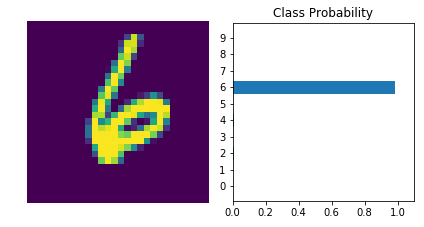
With the network trained, we can check out it's predictions.

images, labels = next(iter(data_loader))

image = images[0].view(1, 784)
# Turn off gradients to speed up this part
with torch.no_grad():
    logits = model.forward(image)

# Output of the network are logits, need to take softmax for probabilities
probabilities = F.softmax(logits, dim=1)
helper.view_classify(image.view(1, 28, 28), probabilities)
probabilities.png

print(probabilities.argmax())
tensor(6)

Amazingly, it did really well. One thing to note is that I originally made the epoch count higher but didn't remember to make a new network, optimizer, and loss, and the network ended up doing poorly. I don't know what messed it up, maybe I reset the network but not the optimizers, or some such, but anyway, here it is.
Backpropagation Implementation (Again)

This is an example of implementing back-propagation using the UCLA Student Admissions data that we used earlier for training with gradient descent.

Set Up

Imports

Python

import itertools

PyPi

from graphviz import Graph
from sklearn.model_selection import train_test_split
from sklearn.preprocessing import scale
import numpy
import pandas

This Project

from neurotic.tangles.data_paths import DataPath
from neurotic.tangles.helpers import org_table

Set the Random Seed

numpy.random.seed(21)

Helper Functions

Once again, the sigmoid.

def sigmoid(x):
    """
    Calculate sigmoid
    """
    return 1 / (1 + numpy.exp(-x))

The Data

We are using data originally take from the UCLA Institute for Digital Research and Education representing a group of students who applied for grad school at UCLA.

path = DataPath("student_data.csv")
data = pandas.read_csv(path.from_folder)
print(org_table(data.head()))
admit gre gpa rank
0 380 3.61 3
1 660 3.67 3
1 800 4 1
1 640 3.19 4
0 520 2.93 4

Pre-Processing the Data

Dummy Variables

Since the rank values are ordinal, not numeric, we need to create some one-hot-encoded columns for it using get_dummies.

rank_counts = data["rank"].value_counts()
data = pandas.get_dummies(data, columns=["rank"], prefix="rank")
for rank in range(1, 5):
    assert rank_counts[rank] == data["rank_{}".format(rank)].sum()
print(org_table(data.head()))
admit gre gpa rank_1 rank_2 rank_3 rank_4
0 380 3.61 0 0 1 0
1 660 3.67 0 0 1 0
1 800 4 1 0 0 0
1 640 3.19 0 0 0 1
0 520 2.93 0 0 0 1

Standardization

Now I'll convert the gre and gpa to have a mean of 0 and a variance of 1 using sklearn's scale function.

data["gre"] = scale(data.gre.astype("float64").values)
data["gpa"] = scale(data.gpa.values)
print(org_table(data.sample(5), showindex=True))
  admit gre gpa rank_1 rank_2 rank_3 rank_4
72 0 -0.933502 0.000263095 0 0 0 1
358 1 -0.240093 0.789548 0 0 1 0
187 0 -0.0667406 -1.34152 0 1 0 0
93 0 -0.0667406 -1.20997 0 1 0 0
380 0 0.973373 0.68431 0 1 0 0
assert data.gre.mean().round() == 0
assert data.gre.std().round() == 1
assert data.gpa.mean().round() == 0
assert data.gpa.std().round() == 1

Setting up the training and testing data

features_all is the input (x) data and targets_all is the target (y) data.

features_all = data.drop("admit", axis="columns")
targets_all = data.admit

Now we'll split it into training and testing sets.

features, features_test, targets, targets_test = train_test_split(
    features_all, targets_all, test_size=0.1)

The Algorithm

These are the basic steps to train the network with backpropagation.

  • Set the weights for each layer to 0
    • Input to hidden weights: \(\Delta w_{ij} = 0\)
    • Hidden to output weights: \(\Delta W_j=0\)
  • For each entry in the training data:
    • make a forward pass to get the output: \(\hat{y}\)
    • Calculate the error gradient for the output: \(\delta^o=(y - \hat{y})f'(\sum_j W_j a_j)\)
    • Propagate the errors to the hidden layer: \(\delta_j^h = \delta^o W_j f'(h_j)\)
    • Update the weight steps:
      • \(\Delta W_j = \Delta W_j + \delta^o a_j\)
      • \(\Delta w_{ij} = \Delta w_{ij} + \delta_j^h a_i\)
  • Update the weights (\(\eta\) is the learning rate and m is the number of records)
    • \(W_j = W_j + \eta \Delta W_j/m\)
    • \(w_{ij} = w_{ij} + \eta \Delta w_{ij}/m\)
  • Repeat for \(\epsilon\) epochs

Hyperparameters

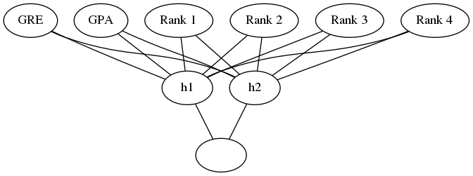
These are the hyperparameters that we set to define the training. We're going to use 2 hidden units.

graph = Graph(format="png")

# the input layer
graph.node("a", "GRE")
graph.node("b", "GPA")
graph.node("c", "Rank 1")
graph.node("d", "Rank 2")
graph.node("e", "Rank 3")
graph.node("f", "Rank 4")

# the hidden layer
graph.node("g", "h1")
graph.node("h", "h2")

# the output layer
graph.node("i", "")

inputs = "abcdef"
hidden = "gh"

graph.edges([x + h for x, h in itertools.product(inputs, hidden)])
graph.edges([h + "i" for h in hidden])

graph.render("graphs/network.dot")
graph

network.dot.png

Well train it for 2,000 epochs with a learning rate of 0.005.

n_hidden = 2
epochs = 2000
learning_rate = 0.005

We'll be using the n_records, and n_features to set up the weights matrices. n_records is also used to average out the amount of change we make to the weights (otherwise each weight would get the sum of all the corrections). last_loss is used for reporting epochs that do worse than the previous epoch.

n_records, n_features = features.shape
last_loss = None

Initialize the Weights

We're going to use a normally distributed set of random weights to start with. The scale is the spread of the distribution we're sampling from. A rule-of-thumb for the spread is to use \(\frac{1}{\sqrt{n}}\) where n is the numeber of input units. This keeps the input to the sigmoid low, even as the number of inputs goes up.

weights_input_to_hidden = numpy.random.normal(scale=1 / n_features ** .5,
                                           size=(n_features, n_hidden))
weights_hidden_to_output = numpy.random.normal(scale=1 / n_features ** .5,
                                            size=n_hidden)

Train It

Now, we'll train the network using backpropagation.

for epoch in range(epochs):
    delta_weights_input_to_hidden = numpy.zeros(weights_input_to_hidden.shape)
    delta_weights_hidden_to_output = numpy.zeros(weights_hidden_to_output.shape)
    for x, y in zip(features.values, targets):
        hidden_input = x.dot(weights_input_to_hidden)
        hidden_output = sigmoid(hidden_input)
        output = sigmoid(hidden_output.dot(weights_hidden_to_output))

        ## Backward pass ##
        error = y - output
        output_error_term = error * output * (1 - output)

        hidden_error = (weights_hidden_to_output.T
                        * output_error_term)
        hidden_error_term = (hidden_error
                             *  hidden_output * (1 - hidden_output))

        delta_weights_hidden_to_output += output_error_term * hidden_output
        delta_weights_input_to_hidden += hidden_error_term * x[:, None]

    weights_input_to_hidden += (learning_rate * delta_weights_input_to_hidden)/n_records
    weights_hidden_to_output += (learning_rate * delta_weights_hidden_to_output)/n_records

    # Printing out the mean square error on the training set
    if epoch % (epochs / 10) == 0:
        hidden_output = sigmoid(numpy.dot(x, weights_input_to_hidden))
        out = sigmoid(numpy.dot(hidden_output,
                             weights_hidden_to_output))
        loss = numpy.mean((out - targets) ** 2)

        if last_loss and last_loss < loss:
            print("Train loss: ", loss, "  WARNING - Loss Increasing")
        else:
            print("Train loss: ", loss)
        last_loss = loss
Train loss:  0.2508914323518061
Train loss:  0.24921862835632544
Train loss:  0.24764092608110996
Train loss:  0.24615251717689884
Train loss:  0.24474791403688867
Train loss:  0.24342194353528698
Train loss:  0.24216973842045766
Train loss:  0.24098672692610631
Train loss:  0.23986862108158177
Train loss:  0.2388114041271259

Now we'll calculate the accuracy of the model.

hidden = sigmoid(numpy.dot(features_test, weights_input_to_hidden))
out = sigmoid(numpy.dot(hidden, weights_hidden_to_output))
predictions = out > 0.5
accuracy = numpy.mean(predictions == targets_test)
print("Prediction accuracy: {:.3f}".format(accuracy))
Prediction accuracy: 0.750

More Backpropagation Reading

Backpropagation

Background

We're going to extend the backpropagation from a single layer to multiple hidden layers. The amount of change at each layer (the delta) that you make uses the same equation no matter how many layers you have.

\[ \Delta w_{pq} = \eta \delta_{output} X_{in} \]

Imports

We'll be sticking with our numpy-based implementation of a neural network.

import numpy

The Sigmoid

This is our familiar activation function.

def sigmoid(x: numpy.ndarray) -> numpy.ndarray:
    """
    Calculate sigmoid
    """
    return 1 / (1 + numpy.exp(-x))

Initial Values

We're going to do a single forward pass followed by backpropagation, so I'll make the values random since we're not really going to validate them..

numpy.random.seed(18)
x = numpy.random.randn(3)
target = numpy.random.random()
learning_rate = numpy.random.random()

weights_input_to_hidden = numpy.random.random((3, 2))
weights_hidden_to_output = numpy.random.random((2, 1))
Variable Value
x [ 0.08 2.19 -0.13]
y 0.85
eta 0.75
Input Weights [0.67 0.99]
  [0.26 0.03]
  [0.64 0.85]
Hidden To Output Weights [0.74]
  [0.02]

The input has 3 nodes and the hidden layer has 2, so our weights from the input layer to the hidden layer has shape 3 rows and 2 columns. The output has one node so the weights from the hidden to output layer has 2 rows (to match the hidden layer) and 1 column to match the output layer. In the lecture they use a vector with 2 entries instead. As far as I can tell it works the same either way.

Forward pass

hidden_layer_input = x.dot(weights_input_to_hidden)
hidden_layer_output = sigmoid(hidden_layer_input)

output_layer_in = hidden_layer_output.dot(weights_hidden_to_output)
output = sigmoid(output_layer_in)

Backwards pass

The Output Error

Our error is \(y - \hat{y}\).

error = target - output

Output Error Term

Our output error term:

\begin{align} \textit{output error term} &= (y - \hat{y}) \times (\hat{y} \times \sigma'(x))\\ &= error \times \hat{y} \times (1 - \hat{y}) \end{align}
output_error_term = error * output * (1 - output)

The Hidden Layer Error Term

The hidden layer error term is the output error term scaled by the weight between them times the derivative of the activation function.

\[ \delta^h = W\delta^o f'(h)\\ \]

hidden_error_term = (weights_hidden_to_output.T
                     * output_error_term
                     * hidden_layer_output * (1 - hidden_layer_output))

The Hidden To Output Weight Update

\[ \Delta W = \eta \delta^o a \]

Where a is the output of the hidden layer.

delta_w_h_o = learning_rate * output_error_term * hidden_layer_output

The Input To Hidden Weight Update

\[ \Delta w_i = \eta \delta^h x_i \]

The update is the learning rate times the hidden unit error times the input values.

delta_w_i_h = learning_rate * hidden_error_term * x[:, None]
print('Change in weights for hidden layer to output layer:')
print(delta_w_h_o)
print('Change in weights for input layer to hidden layer:')
print(delta_w_i_h)
Change in weights for hidden layer to output layer:
[0.02634231 0.02119776]
Change in weights for input layer to hidden layer:
[[ 5.70726224e-04  1.72873580e-05]
 [ 1.57375099e-02  4.76690849e-04]
 [-9.69255871e-04 -2.93588634e-05]]

Multi-Layer Perceptrons

This is basically like the previous gradient-descent post but with more layers.

Set Up

Imports

From PyPi

from graphviz import Graph
import numpy

The Activation Function

def sigmoid(x):
    """
    Calculate sigmoid
    """
    return 1/(1 + numpy.exp(-x))

Defining Our Network

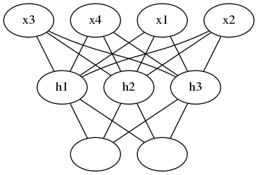
These variables will define our network size.

N_input = 4
N_hidden = 3
N_output = 2

Which produces a network like this.

graph = Graph(format="png")

# input layer
graph.node("a", "x1")
graph.node("b", "x2")
graph.node("c", "x3")
graph.node("d", "x4")

# hidden layer
graph.node("e", "h1")
graph.node("f", "h2")
graph.node("g", "h3")

# output layer
graph.node("h", "")
graph.node("i", "")

graph.edges(["ae", "af", "ag", "be", "bf", "bg", "ce", "cf", "cg", "de", "df", "dg"])
graph.edges(["eh", "ei", "fh", "fi", "gh", "gi"])

graph.render("graphs/network.dot")
graph

network.dot.png

Next, set the random seed.

numpy.random.seed(42)

Some fake data to train on.

X = numpy.random.randn(4)
print(X.shape)
(4,)

Now initialize our weights.

weights_input_to_hidden = numpy.random.normal(0, scale=0.1, size=(N_input, N_hidden))
weights_hidden_to_output = numpy.random.normal(0, scale=0.1, size=(N_hidden, N_output))
print(weights_input_to_hidden.shape)
print(weights_hidden_to_output.shape)
(4, 3)
(3, 2)

Forward Pass

This is one forward pass through our network.

hidden_layer_in = X.dot(weights_input_to_hidden)
hidden_layer_out = sigmoid(hidden_layer_in)
print('Hidden-layer Output:')
print(hidden_layer_out)
Hidden-layer Output:
[0.5609517  0.4810582  0.44218495]

Now our output.

output_layer_in = hidden_layer_out.dot(weights_hidden_to_output)
output_layer_out = sigmoid(output_layer_in)
print('Output-layer Output:')
print(output_layer_out)
Output-layer Output:
[0.49936449 0.46156347]

Training with Gradient Descent

This is an example of implementing gradient descent to update the weights in a neural network.

Set Up

Imports

From PyPi

from sklearn.model_selection import train_test_split
from sklearn.preprocessing import scale
import matplotlib.pyplot as pyplot
import numpy
import pandas
import seaborn

This Project

from neurotic.tangles.data_paths import DataPath
from neurotic.tangles.helpers import org_table

Plotting

%matplotlib inline
seaborn.set(style="whitegrid",
            rc={"axes.grid": False,
                "font.family": ["sans-serif"],
                "font.sans-serif": ["Latin Modern Sans", "Lato"],
                "figure.figsize": (20, 40)},
            font_scale=2)
FIGURE_SIZE = (12, 10)

The Data

We will use data originally take from the UCLA Institute for Digital Research and Education (I couldn't find the dataset when I went to look for it). It has three features:

Feature Description
gre Graduate Record Exam score
gpa Grade Point Average
rank Rank of the undergraduate school

The rank is a scale from 1 to 4, with 1 being the most prestigious school and 4 being the least.

It also has one output value - admit which indicates whether the student was admitted or not.

path = DataPath("student_data.csv")
data = pandas.read_csv(path.from_folder)
print(org_table(data.head()))
admit gre gpa rank
0 380 3.61 3
1 660 3.67 3
1 800 4 1
1 640 3.19 4
0 520 2.93 4
print(data.shape)
(400, 7)

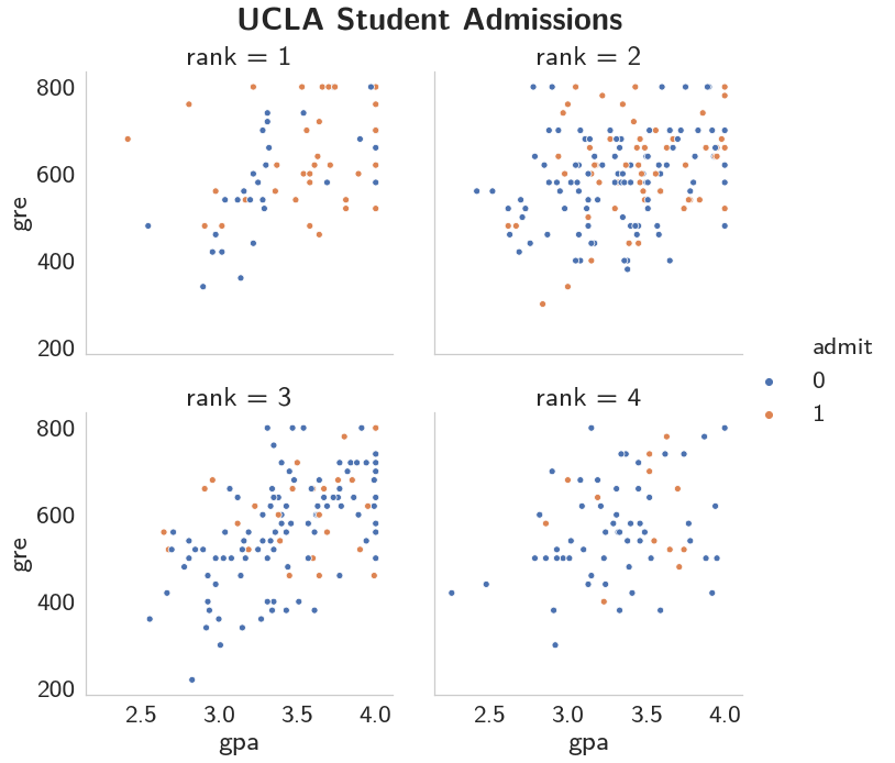
So there are 400 applications - not a huge data set.

grid = seaborn.relplot(x="gpa", y="gre", hue="admit", col="rank",
                       data=data, col_wrap=2)
pyplot.subplots_adjust(top=0.9)
title = grid.fig.suptitle("UCLA Student Admissions", weight="bold")

admissions.png

It does look like the rank of the school matters, perhaps even more than scores.

with seaborn.color_palette("PuBuGn_d"):
    grid = seaborn.catplot(x="rank", kind="count", data=data,
                           height=10, aspect=12/10)
    title = grid.fig.suptitle("UCLA Student Submissions By Rank", weight="bold")

rank_distribution.png

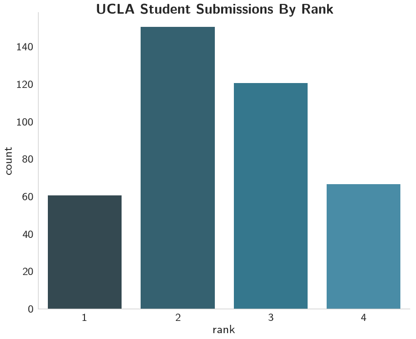
So most of the applicants came from second and third-ranked schools.

admitted = data[data.admit==1]
with seaborn.color_palette("PuBuGn_d"):
    grid = seaborn.catplot(x="rank", kind="count", data=admitted,
                           height=10, aspect=12/10)
    title = grid.fig.suptitle("UCLA Student Admissions By Rank",
                              weight="bold")

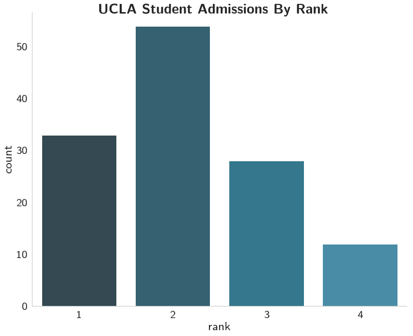
admitted_ranks.png And it looks like most of the admitted were from first and second-ranked schools, with most coming from the second-ranked schools.
admission_rate = (admitted["rank"].value_counts(sort=False)
                  /data["rank"].value_counts(sort=False))
admission_rate = (admission_rate * 100).round(2)
admission_rate = admission_rate.reset_index()
admission_rate.columns = ["Rank", "Percent Admitted"]
print(org_table(admission_rate))
Rank Percent Admitted
1 54.1
2 35.76
3 23.14
4 17.91

So, even though the second-tier schools had the most admitted, the top-tier school was admitted at a higher rate.

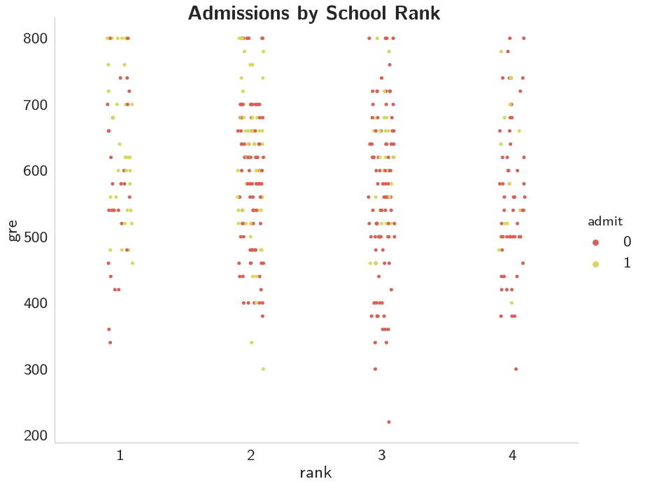
Did GRE Matter?

with seaborn.color_palette("hls"):
    grid = seaborn.catplot(x="rank", y="gre", hue="admit", data=data,
                           height=10, aspect=12/10)
    title = grid.fig.suptitle("Admissions by School Rank", weight="bold")

gre_rank_admissions.png

This one's a little tough to say, it looks like it's better to have a higher GRE, but once you get below 700 it isn't as clear, at least not to me.

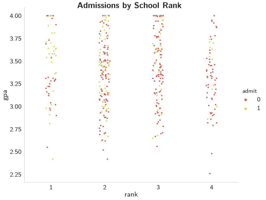
What about GPA?

with seaborn.color_palette("hls"):
    grid = seaborn.catplot(x="rank", y="gpa", hue="admit", data=data,
                           height=10, aspect=12/10)
    title = grid.fig.suptitle("Admissions by School Rank", weight="bold")

gpa_rank_admissions.png

This one seems even less demonstrative than GRE does.

Pre-Processing the Data

Dummy Variables

Since the rank values are ordinal, not numeric, we need to create some one-hot-encoded columns for it using get_dummies.

First I'll get some counts so I can double-check my work. Note to future self: rank is a pandas DataFrame method, so naming a column 'rank' is probably not such a great idea.

rank_counts = data["rank"].value_counts()
data = pandas.get_dummies(data, columns=["rank"], prefix="rank")
for rank in range(1, 5):
    assert rank_counts[rank] == data["rank_{}".format(rank)].sum()
print(org_table(data.head()))
admit gre gpa rank_1 rank_2 rank_3 rank_4
0 380 3.61 0 0 1 0
1 660 3.67 0 0 1 0
1 800 4 1 0 0 0
1 640 3.19 0 0 0 1
0 520 2.93 0 0 0 1

Standardization

Now I'll convert the gre and gpa to have a mean of 0 and a variance of 1 using sklearn's scale function.

data["gre"] = scale(data.gre.astype("float64").values)
data["gpa"] = scale(data.gpa.values)
print(org_table(data.sample(5)))
admit gre gpa rank_1 rank_2 rank_3 rank_4
0 -0.240093 -0.394379 0 0 0 1
1 0.973373 1.60514 1 0 0 0
0 -0.413445 -0.0260464 0 0 0 1
1 0.106612 -0.631165 0 1 0 0
0 -0.760149 -1.52569 0 0 1 0
print(data.gre.mean().round())
print(data.gre.std().round())
print(data.gpa.mean().round())
print(data.gpa.std().round())
-0.0
1.0
0.0
1.0

The Error

For this we're going to use the Mean Square Error.

\[ E = \frac{1}{2m}\sum_{\mu} (y^{\mu} - \hat{y}^{\mu})^2 \]

This doesn't actually change our training, it just acts as an estimate of the error as we train so we can see that the model is getting better (hopefully).

The General Training Algorithm

  • Set the weight delta to 0 (\(\Delta w_i = 0\))
  • For each record in the training data:
    • Make a forward pass to get the output: \(\hat{y} = f\left(\sum_{i} w_i x_i \right)\)
    • Calculate the error: \(\delta = (y - \hat{y}) f'\left(\sum_i w_i x_i\right)\)
    • Update the weight delta: \(\Delta w_i = \Delta w_i + \delta x_i\)
  • Update the weights : \(w_i = w_i + \eta \frac{\Delta w_i}{m}\)
  • Repeart for \(e\) epochs

The Numpy Implementation

I'm going to implement the previous algorithm using numpy.

Setting up the Data

We need to set up the training and testing data. The lecture uses numpy exclusively, but as with the standardization I'll cheat a little and use sklearn. The lecture uses a slightly different naming scheme from the one you normally see in the python machine learning community (e.g. X_train, y_train) which I'll stick with it so that I don't get errors just from using the wrong names. Truthfully, I kind of like these names better, although the use of the suffix _test without the use of the suffix _train seems confusing.

features_all = data.drop("admit", axis="columns")
targets_all = data.admit

The example given uses 10 % of the data for testing and 90% for training.

features, features_test, targets, targets_test = train_test_split(features_all, targets_all, test_size=0.1)
print(features.shape)
print(targets.shape)
print(features_test.shape)
print(targets_test.shape)
(360, 6)
(360,)
(40, 6)
(40,)

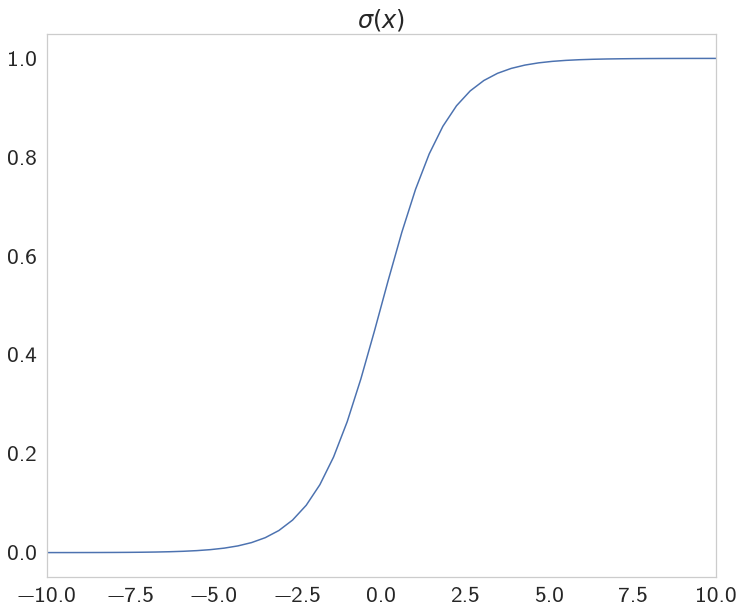
The Sigmoid

This is our activation function.

def sigmoid(x):
    """
    Calculate sigmoid
    """
    return 1 / (1 + numpy.exp(-x))
limit = [-10, 10]
x = numpy.linspace(*limit)
y = sigmoid(x)
figure, axe = pyplot.subplots(figsize=FIGURE_SIZE)
axe.set_xlim(*limit)
axe.set_title("$\sigma(x)$", weight="bold")
plot = axe.plot(x, y)

sigmoid.png

Some Setup

To make the outcome reproducible I'll set the random seed.

numpy.random.seed(17)

Now some variables need to be set up for the print output.

n_records, n_features = features.shape
last_loss = None

Initialize weights

We're going to use a normally distributed set of random weights to start with. The scale is the spread of the distribution we're sampling from. A rule-of-thumb for the spread is to use \(\frac{1}{\sqrt{n}}\) where n is the numeber of input units. This keeps the input to the sigmoid low, even as the number of inputs goes up.

weights = numpy.random.normal(scale=1/n_features**.5, size=n_features)

Set Up The Learning

Now some neural network hyperparameters - how long do we train and how fast do we learn at each pass?

epochs = 1000
learnrate = 0.5

The Training Loop

This is where we do the actual training (gradient descent).

for epoch in range(epochs):
    delta_weights = numpy.zeros(weights.shape)
    for x, y in zip(features.values, targets):
        output = sigmoid(x.dot(weights))

        error = y - output

        error_term = error * (output * (1 - output))

        delta_weights += error_term * x

    weights += (learnrate * delta_weights)/n_records

    # Printing out the mean square error on the training set
    if epoch % (epochs / 10) == 0:
        out = sigmoid(numpy.dot(features, weights))
        loss = numpy.mean((out - targets) ** 2)
        if last_loss and last_loss < loss:
            print("Train loss: ", loss, "  WARNING - Loss Increasing")
        else:
            print("Train loss: ", loss)
        last_loss = loss
Train loss:  0.31403028569037034
Train loss:  0.20839043233748233
Train loss:  0.19937544110681996
Train loss:  0.19697280538767817
Train loss:  0.19607622516320752
Train loss:  0.19567788493090374
Train loss:  0.19548034981121246
Train loss:  0.19537454797678722
Train loss:  0.19531455174429538
Train loss:  0.19527902197312702

Testing

Calculate accuracy on test data

test_out = sigmoid(numpy.dot(features_test, weights))
predictions = test_out > 0.5
accuracy = numpy.mean(predictions == targets_test)
print("Prediction accuracy: {:.3f}".format(accuracy))
Prediction accuracy: 0.750

Not great, but then again, we had a fairly small data set to start with.

Gradient Descent (Again)

Table of Contents

Some Math

One weight update for gradient descent is calculated as:

\[ \Delta w_i = \eta \delta x_i \]

And the error term \(\delta\) is calculated as:

\begin{align} \delta &= (y - \hat{y}) f'(h)\\ &= (y - \hat{y})f'\left(\sum w_i x_i\right) \end{align}

If we are using the sigmoid activation function as \(f(x)\):

\[ \sigma(x) = \frac{1}{1 - e^{-x}} \]

Then its derivative \(f'(x)\) is:

\[ \sigma(x) (1 - \sigma(x)) \]

An Implementation

Imports

import numpy

The Sigmoid

def sigmoid(x): numpy.ndarray -> numpy.ndarray:
    """
    Our activation function

    Args:
     x: the input array

    Returns:
     the sigmoid of x
    """
    return 1/(1 + numpy.exp(-x))

The Sigmoid Derivative

def sigmoid_prime(x: numpy.ndarray) -> numpy.ndarray:
    """
    The derivative of the sigmoid

    Args:
     x: the input

    Returns:
     the sigmoid derivative of x
    """
    return sigmoid(x) * (1 - sigmoid(x))

Setup The Network

learning_rate = 0.5
x = numpy.array([1, 2, 3, 4])
y = numpy.array(0.5)

# Initial weights
w = numpy.array([0.5, -0.5, 0.3, 0.1])

The Network

This will calculate a single gradient descent step.

The Fordward pass

hidden_layer = x.dot(w)
y_hat = sigmoid(hidden_layer)

Backwards Propagation

error = y - y_hat

error_term = error * sigmoid_prime(hidden_layer)

delta_w = learning_rate * error_term * x

print('Neural Network output:')
print(y_hat)
print('Amount of Error:')
print(error)
print('Change in Weights:')
print(delta_w)
Neural Network output:
0.6899744811276125
Amount of Error:
-0.1899744811276125
Change in Weights:
[-0.02031869 -0.04063738 -0.06095608 -0.08127477]

Part 2 - Neural Networks in Pytorch

Introduction

Deep learning networks tend to be massive with dozens or hundreds of layers, that's where the term "deep" comes from. You can build one of these deep networks using only weight matrices as we did in the previous notebook, but in general it's very cumbersome and difficult to implement. PyTorch has a nice module nn that provides a nice way to efficiently build large neural networks.

Set Up

Python

from collections import OrderedDict

Imports

PyPi

from torch import nn
import matplotlib.pyplot as pyplot
import numpy
import seaborn
import torch

From the Nano-Degree Repository

from nano.pytorch import helper

Plotting

get_python().run_line_magic('matplotlib', 'inline')
get_python().run_line_magic('config', "InlineBackend.figure_format = 'retina'")
seaborn.set(style="whitegrid",
            rc={"axes.grid": False,
                "font.family": ["sans-serif"],
                "font.sans-serif": ["Latin Modern Sans", "Lato"],
                "figure.figsize": (8, 6)},
            font_scale=2)

The First Network

Now we're going to build a larger network that can solve a (formerly) difficult problem, identifying text in an image. Here we'll use the MNIST dataset which consists of greyscale handwritten digits. Each image is 28x28 pixels. Our goal is to build a neural network that can take one of these images and predict the digit in the image.

First up, we need to get our dataset. This is provided through the torchvision package. The code below will download the MNIST dataset, then create training and test datasets for us. Don't worry too much about the details here, you'll learn more about this later. (see torchvision.dataset and torchvision.transforms).

from torchvision import datasets, transforms

Transformers:

  • transforms.compose lets you set up multiple transforms in a pipeline.
  • transforms.Normalize normalizes images using the mean and standard deviation.
  • transforms.ToTensor converts images to Tensors.

Define a transform to normalize the data.

transform = transforms.Compose([transforms.ToTensor(),
                              transforms.Normalize((0.5, 0.5, 0.5), (0.5, 0.5, 0.5)),
                              ])

Download and load the training data

torch.utils.data.DataLoader builds an iterator over the data.

trainset = datasets.MNIST('~/datasets/MNIST/', download=True, train=True, transform=transform)
trainloader = torch.utils.data.DataLoader(trainset, batch_size=64, shuffle=True)

The data-set isn't actually part of pytorch, it just downloads it from the web (unless you already downloaded it).

Downloading http://yann.lecun.com/exdb/mnist/train-images-idx3-ubyte.gz
Downloading http://yann.lecun.com/exdb/mnist/train-labels-idx1-ubyte.gz
Downloading http://yann.lecun.com/exdb/mnist/t10k-images-idx3-ubyte.gz
Downloading http://yann.lecun.com/exdb/mnist/t10k-labels-idx1-ubyte.gz
Processing...
Done!

We have the training data loaded into trainloader and we make that an iterator with iter(trainloader). Later, we'll use this to loop through the dataset for training, something like:

for image, label in trainloader:
    do things with images and labels

The trainloader has a batch size of 64, and shuffle=True. The batch size is the number of images we get in one iteration from the data loader and pass through our network, often called a batch. And shuffle=True tells it to shuffle the dataset every time we start going through the data loader again. But here I'm just grabbing the first batch so we can check out the data. We can see below that images is just a tensor with size (64, 1, 28, 28). So, 64 images per batch, 1 color channel, and 28x28 images.

dataiter = iter(trainloader)
images, labels = dataiter.next()
print(type(images))
print(images.shape)
print(labels.shape)
<class 'torch.Tensor'>
torch.Size([64, 1, 28, 28])
torch.Size([64])

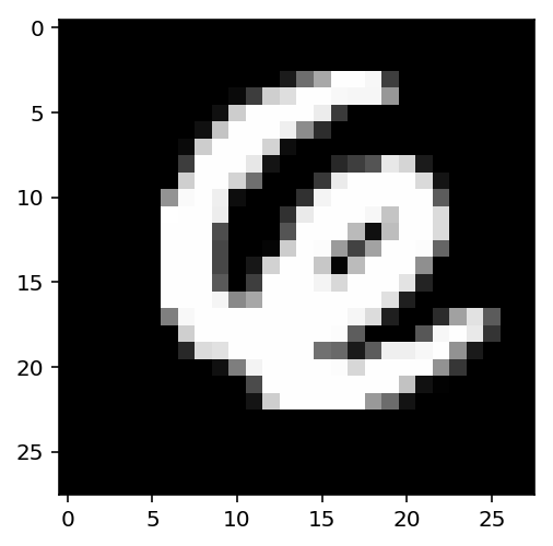
Here's what one of the images looks like.

pyplot.imshow(images[1].numpy().squeeze(), cmap='Greys_r');

image.png

Can you tell what that is? I couldn't, so I looked it up.

print(labels[1])
tensor(6)

First, let's try to build a simple network for this dataset using weight matrices and matrix multiplications. Then, we'll see how to do it using PyTorch's nn module which provides a much more convenient and powerful method for defining network architectures.

Flattening The Input

The networks you've seen so far are called fully-connected or dense networks. Each unit in one layer is connected to each unit in the next layer. In fully-connected networks, the input to each layer must be a one-dimensional vector (which can be stacked into a 2D tensor as a batch of multiple examples). However, our images are 28x28 2D tensors, so we need to convert them into 1D vectors. Thinking about sizes, we need to convert the batch of images with shape `(64, 1, 28, 28)` to a have a shape of `(64, 784)`, 784 is 28 times 28. This is typically called flattening, we flattened the 2D images into 1D vectors.

Previously you built a network with one output unit. Here we need 10 output units, one for each digit. We want our network to predict the digit shown in an image, so what we'll do is calculate probabilities that the image is of any one digit or class. This ends up being a discrete probability distribution over the classes (digits) that tells us the most likely class for the image. That means we need 10 output units for the 10 classes (digits). We'll see how to convert the network output into a probability distribution next.

Now we're going to flatten the batch of images images then build a multi-layer network with 784 input units, 256 hidden units, and 10 output units using random tensors for the weights and biases. It will use a sigmoid activation for the hidden layer and no activation function for the output layer.

out = torch.randn(64, 10)
assert out.shape == torch.Size([64, 10])

Now we have 10 outputs for our network. We want to pass in an image to our network and get out a probability distribution over the classes that tells us the likely class(es) the image belongs to.

For an untrained network that hasn't seen any data yet the output probability distribution will be a uniform distribution with equal probabilities for each class.

To calculate this probability distribution, we often use the softmax function. Mathematically this looks like

\[ \Large \sigma(x_i) = \cfrac{e^{x_i}}{\sum_k^K{e^{x_k}}} \]

What this does is squish each input \(x_i\) between 0 and 1 and normalizes the values to give you a proper probability distribution where the probabilites sum up to one.

Softmax Implementation

Implement a function softmax that performs the softmax calculation and returns probability distributions for each example in the batch. Note that you'll need to pay attention to the shapes when doing this. If you have a tensor a with shape (64, 10) and a tensor b with shape (64,), doing a/b will give you an error because PyTorch will try to do the division across the columns (called broadcasting) but you'll get a size mismatch. The way to think about this is for each of the 64 examples, you only want to divide by one value, the sum in the denominator. So you need b to have a shape of (64, 1). This way PyTorch will divide the 10 values in each row of a by the one value in each row of b. Pay attention to how you take the sum as well. You'll need to define the dim keyword in torch.sum. Setting dim=0 takes the sum across the rows while dim=1 takes the sum across the columns.

def softmax(x: numpy.ndarray) -> numpy.ndarray:
    """Calculates the softmax"""
    numerator = torch.exp(x)
    denominator = numerator.sum(dim=1).view(64, 1)
    return numerator/denominator

Here, out should be the output of the network in the previous excercise with shape (64,10)

probabilities = softmax(out)

Does it have the right shape? Should be (64, 10)

assert probabilities.shape == out.shape
print(probabilities.shape)
torch.Size([64, 10])

Does it sum to 1?

expected = numpy.ones(64)
actual = probabilities.sum(dim=1)
print(actual)
assert numpy.allclose(expected, actual)
tensor([1.0000, 1.0000, 1.0000, 1.0000, 1.0000, 1.0000, 1.0000, 1.0000, 1.0000,
        1.0000, 1.0000, 1.0000, 1.0000, 1.0000, 1.0000, 1.0000, 1.0000, 1.0000,
        1.0000, 1.0000, 1.0000, 1.0000, 1.0000, 1.0000, 1.0000, 1.0000, 1.0000,
        1.0000, 1.0000, 1.0000, 1.0000, 1.0000, 1.0000, 1.0000, 1.0000, 1.0000,
        1.0000, 1.0000, 1.0000, 1.0000, 1.0000, 1.0000, 1.0000, 1.0000, 1.0000,
        1.0000, 1.0000, 1.0000, 1.0000, 1.0000, 1.0000, 1.0000, 1.0000, 1.0000,
        1.0000, 1.0000, 1.0000, 1.0000, 1.0000, 1.0000, 1.0000, 1.0000, 1.0000,
        1.0000])

Building networks with PyTorch

PyTorch provides a module nn that makes building networks much simpler. Here I'll show you how to build the same one as above with 784 inputs, 256 hidden units, 10 output units and a softmax output.

The Class Definition

class Network(nn.Module):
    def __init__(self):
        super().__init__()

        # Inputs to hidden layer linear transformation
        self.hidden = nn.Linear(784, 256)
        # Output layer, 10 units - one for each digit
        self.output = nn.Linear(256, 10)

        # Define sigmoid activation and softmax output 
        self.sigmoid = nn.Sigmoid()
        self.softmax = nn.Softmax(dim=1)

    def forward(self, x):
        # Pass the input tensor through each of our operations
        x = self.hidden(x)
        x = self.sigmoid(x)
        x = self.output(x)
        x = self.softmax(x)
        return x

Let's go through this bit by bit.

Inherit from nn.Module

class Network(nn.Module):

Here we're inheriting from nn.Module. Combined with super().__init__() this creates a class that tracks the architecture and provides a lot of useful methods and attributes. It is mandatory to inherit from nn.Module when you're creating a class for your network. The name of the class itself can be anything.

The Hidden Layer

self.hidden = nn.Linear(784, 256)

This line creates a module for a linear transformation, \(x\mathbf{W} + b\), with 784 inputs and 256 outputs and assigns it to self.hidden. The module automatically creates the weight and bias tensors which we'll use in the forward method. You can access the weight and bias tensors once the network once it's create at net.hidden.weight and net.hidden.bias.

The Output Layer

self.output = nn.Linear(256, 10)

Similarly, this creates another linear transformation with 256 inputs and 10 outputs.

The Activation Layers

self.sigmoid = nn.Sigmoid()
self.softmax = nn.Softmax(dim=1)

Next we set up our sigmoid activation method and softmax output method. The argument dim tells it which axis to use. Setting it to 1 tells it to sum the columns, so you will end up with 1 entry for every row.

The Forward-Pass Method

def forward(self, x):

PyTorch networks created with nn.Module must have a forward method defined. It takes in a tensor x and passes it through the operations you defined in the __init__ method.

x = self.hidden(x)
x = self.sigmoid(x)
x = self.output(x)
x = self.softmax(x)

Here the input tensor x is passed through each operation and reassigned to x. We can see that the input tensor goes through the hidden layer, then a sigmoid function, then the output layer, and finally the softmax function. It doesn't matter what you name the variables here, as long as the inputs and outputs of the operations match the network architecture you want to build. The order in which you define things in the __init__ method doesn't matter, but you'll need to sequence the operations correctly in the forward method.

Instantiating the Model

Now we can create a Network object.

Here's what the text representation for an instance looks like.

model = Network()
print(model)
Network(
  (hidden): Linear(in_features=784, out_features=256, bias=True)
  (output): Linear(in_features=256, out_features=10, bias=True)
  (sigmoid): Sigmoid()
  (softmax): Softmax()
)

You can define the network somewhat more concisely and clearly using the torch.nn.functional module. This is the most common way you'll see networks defined as many operations are simple element-wise functions. We normally import this module as F, import torch.nn.functional as F.

import torch.nn.functional as F

class Network(nn.Module):
    def __init__(self):
        super().__init__()
        # Inputs to hidden layer linear transformation
        self.hidden = nn.Linear(784, 256)
        # Output layer, 10 units - one for each digit
        self.output = nn.Linear(256, 10)

    def forward(self, x):
        # Hidden layer with sigmoid activation
        x = F.sigmoid(self.hidden(x))
        # Output layer with softmax activation
        x = F.softmax(self.output(x), dim=1)        
        return x

Activation functions

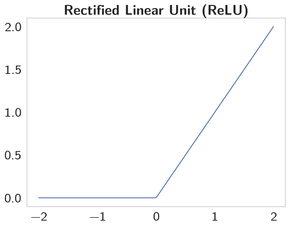
So far we've only been looking at the softmax activation, but in general any function can be used as an activation function. The only requirement is that for a network to approximate a non-linear function, the activation functions must be non-linear. Here are a few more examples of common activation functions: Tanh (hyperbolic tangent), and ReLU (rectified linear unit).

In practice, the ReLU function is used almost exclusively as the activation function for hidden layers.

Let's Build a Network

We're going to create a network with 784 input units, a hidden layer with 128 units and a ReLU activation, then a hidden layer with 64 units and a ReLU activation, and finally an output layer with a softmax activation as shown above. You can use a ReLU activation with the nn.ReLU module or F.relu function.

figure, axe = pyplot.subplots()
x = numpy.linspace(-2, 2, num=200)
y = [max(0, element) for element in x]
axe.set_title("Rectified Linear Unit (ReLU)", weight="bold")
plot = axe.plot(x, y)

relu.png

The ReLU is a function with the form of \(y = max(0, x)\).

We're going to create a network with 784 input units, a hidden layer with 128 units and a ReLU activation, then a hidden layer with 64 units and a ReLU activation, and finally an output layer with a softmax activation as shown above. You can use a ReLU activation with the nn.ReLU module or F.relu function.

class ReluNet(nn.Module):
    """Creates a network with two hidden layers

    Each hidden layer will use ReLU activation
    The output will use softmax activation

    Args:
     inputs: number of input nodes
     hidden_one: number of nodes in the first hidden layer
     hidden_two: number of nodes in the second layer
     outputs: number of nodes in the output layer
    """
    def __init__(self, inputs: int=784,
                 hidden_one: int=128,
                 hidden_two: int=64,
                 outputs: int=10):
        super().__init__()
        self.input_to_hidden_one = nn.Linear(inputs, hidden_one)
        self.hidden_one_to_hidden_two = nn.Linear(hidden_one, hidden_two)
        self.hidden_two_to_output = nn.Linear(hidden_two, outputs)
        self.relu = nn.ReLU()
        self.softmax = nn.Softmax(dim=1)
        return

    def forward(self, x: torch.Tensor) -> torch.Tensor:
        """Does the forward-pass through the network"""
        x = self.relu(self.input_to_hidden_one(x))
        x = self.relu(self.hidden_one_to_hidden_two(x))
        return self.softmax(self.hidden_two_to_output(x))
model = ReluNet()
print(model)
ReluNet(
  (input_to_hidden_one): Linear(in_features=784, out_features=128, bias=True)
  (hidden_one_to_hidden_two): Linear(in_features=128, out_features=64, bias=True)
  (hidden_two_to_output): Linear(in_features=64, out_features=10, bias=True)
  (relu): ReLU()
  (softmax): Softmax()
)

Initializing weights and biases

The weights and such are automatically initialized for you, but it's possible to customize how they are initialized. The weights and biases are tensors attached to the layer you defined, you can get them with model.fc1.weight for instance.

print(model.hidden_one_to_hidden_two.weight)
print(model.hidden_one_to_hidden_two.bias)
Parameter containing:
tensor([[-0.0489, -0.0440, -0.0060,  ..., -0.0246, -0.0269,  0.0096],
        [ 0.0739,  0.0338, -0.0180,  ..., -0.0785, -0.0467, -0.0290],
        [-0.0117, -0.0637,  0.0105,  ...,  0.0158,  0.0126, -0.0255],
        ...,
        [ 0.0077, -0.0302,  0.0320,  ..., -0.0089, -0.0645, -0.0595],
        [-0.0269, -0.0370, -0.0317,  ...,  0.0258,  0.0334,  0.0240],
        [ 0.0227,  0.0195,  0.0731,  ...,  0.0510,  0.0119, -0.0791]],
       requires_grad=True)
Parameter containing:
tensor([-0.0820, -0.0675,  0.0483, -0.0245,  0.0227,  0.0306, -0.0397,  0.0602,
         0.0737, -0.0517, -0.0539,  0.0142,  0.0129, -0.0251,  0.0813,  0.0114,
         0.0445, -0.0508,  0.0709, -0.0684, -0.0822,  0.0084, -0.0751,  0.0594,
        -0.0248,  0.0041,  0.0369, -0.0762, -0.0170,  0.0306, -0.0295, -0.0396,
        -0.0442, -0.0408,  0.0189, -0.0410,  0.0593, -0.0696, -0.0551, -0.0633,
         0.0681,  0.0720,  0.0678,  0.0486,  0.0795, -0.0340,  0.0176,  0.0837,
        -0.0152,  0.0514, -0.0676,  0.0065,  0.0309, -0.0441, -0.0364, -0.0513,
        -0.0145, -0.0328,  0.0282,  0.0612, -0.0549, -0.0411,  0.0456,  0.0129],
       requires_grad=True)

For custom initialization, we want to modify these tensors in place. These are actually autograd Variables, which perform automatic differentiation for us, so we need to get back the actual tensors with model.hidden_one_to_hidden_two.weight.data. Once we have the tensors, we can fill them with zeros (for biases) or random normal values.

Set biases to all zeros:

model.input_to_hidden_one.bias.data.fill_(0)

Sample from random normal with standard dev = 0.01

model.input_to_hidden_one.weight.data.normal_(std=0.01)

Forward pass

Now that we have a network, let's see what happens when we pass in an image.

Grab some data

This next block grabs one batch of image data.

batch = iter(trainloader)
images, labels = batch.next()

Now we need to resize the images into a 1D vector. The new shape is (batch size, color channels, image pixels).

images.resize_(len(images), 1, 28*28)

Forward pass through the network

image = images[0, :]
probabilities = model.forward(image)
highest = probabilities.argmax()
print(highest)
print(probabilities[:, highest])
tensor(2)
tensor([0.1173], grad_fn=<SelectBackward>)

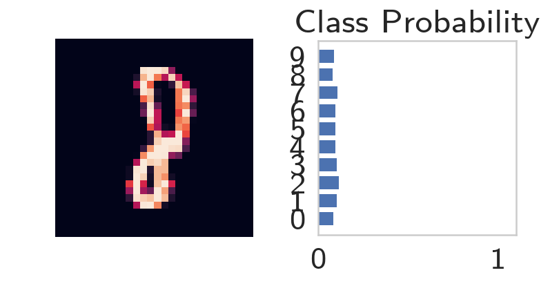
It looks like we're predicting a 2.

helper.view_classify(image.view(1, 28, 28), probabilities)

image_2.png

As you can see above, our network has basically no idea what this digit is. It's because we haven't trained it yet so all the weights are random.

Using nn.Sequential

PyTorch provides a convenient way to build networks like this where a tensor is passed sequentially through operations, nn.Sequential (documentation). This is how you use Sequential to build the equivalent network.

Hyperparameters For Our Network

input_size = 784
hidden_sizes = [128, 64]
output_size = 10

Build a Feed-Forward Network

model = nn.Sequential(nn.Linear(input_size, hidden_sizes[0]),
                      nn.ReLU(),
                      nn.Linear(hidden_sizes[0], hidden_sizes[1]),
                      nn.ReLU(),
                      nn.Linear(hidden_sizes[1], output_size),
                      nn.Softmax(dim=1))
print(model)
Sequential(
  (0): Linear(in_features=784, out_features=128, bias=True)
  (1): ReLU()
  (2): Linear(in_features=128, out_features=64, bias=True)
  (3): ReLU()
  (4): Linear(in_features=64, out_features=10, bias=True)
  (5): Softmax()
)

Forward Pass

images, labels = next(iter(trainloader))
images.resize_(images.shape[0], 1, 784)
image = images[0, :]
probabilities = model.forward(image)
helper.view_classify(image.view(1, 28, 28), probabilities)

image_3.png

The operations are availble by passing in the appropriate index. For example, if you want to get the first Linear operation and look at the weights, you'd use model[0].

print(model[0])
print(model[0].weight)
Linear(in_features=784, out_features=128, bias=True)
Parameter containing:
tensor([[-0.0229,  0.0106,  0.0077,  ...,  0.0079, -0.0073, -0.0182],
        [-0.0066,  0.0245,  0.0241,  ...,  0.0344,  0.0281,  0.0034],
        [-0.0349,  0.0127,  0.0119,  ..., -0.0351,  0.0160,  0.0235],
        ...,
        [-0.0328,  0.0114,  0.0204,  ...,  0.0265, -0.0114,  0.0215],
        [-0.0214, -0.0027, -0.0279,  ..., -0.0297, -0.0112, -0.0189],
        [ 0.0217,  0.0208, -0.0328,  ...,  0.0341,  0.0270, -0.0198]],
       requires_grad=True)

You can also pass in an OrderedDict to name the individual layers and operations, instead of using incremental integers. Note that dictionary keys must be unique, so each operation must have a different name.

model = nn.Sequential(OrderedDict([
                      ('input_to_hidden', nn.Linear(input_size, hidden_sizes[0])),
                      ('relu_1', nn.ReLU()),
                      ('hidden_to_hidden', nn.Linear(hidden_sizes[0], hidden_sizes[1])),
                      ('relu_2', nn.ReLU()),
                      ('output', nn.Linear(hidden_sizes[1], output_size)),
                      ('softmax', nn.Softmax(dim=1))]))
print(model)
Sequential(
  (input_to_hidden): Linear(in_features=784, out_features=128, bias=True)
  (relu_1): ReLU()
  (hidden_to_hidden): Linear(in_features=128, out_features=64, bias=True)
  (relu_2): ReLU()
  (output): Linear(in_features=64, out_features=10, bias=True)
  (softmax): Softmax()
)
print(model[0])
print(model.input_to_hidden)
assert model[0] is model.input_to_hidden
Linear(in_features=784, out_features=128, bias=True)

Inspecting the Weights

Set Up

Imports

Python

import pickle

PyPi

from bokeh.embed import autoload_static
from bokeh.plotting import (
    figure,
    ColumnDataSource,
    )
from bokeh.models import LabelSet
import bokeh.resources
import matplotlib.colors as colors
from sklearn.manifold import TSNE

This Project

from sentiment_noise_reduction import SentimentNoiseReduction
from neurotic.tangles.data_paths import DataPath

What's Going on in the Weights?

Let's start with a model that doesn't have any noise cancellation.

with DataPath("x_train.pkl").from_folder.open("rb") as reader:
    x_train = pickle.load(reader)

with DataPath("y_train.pkl").from_folder.open("rb") as reader:
    y_train = pickle.load(reader)
mlp_full = SentimentNoiseReduction(lower_bound=0,
                                   polarity_cutoff=0,
                                   learning_rate=0.01,
                                   verbose=True)
mlp_full.train(x_train, y_train)
Progress: 0.00 % Speed(reviews/sec): 0.00 Error: [-0.5] #Correct: 1 #Trained: 1 Training Accuracy: 100.00 %
Progress: 4.17 % Speed(reviews/sec): 125.00 Error: [-0.38320156] #Correct: 740 #Trained: 1001 Training Accuracy: 73.93 %
Progress: 8.33 % Speed(reviews/sec): 222.22 Error: [-0.26004622] #Correct: 1529 #Trained: 2001 Training Accuracy: 76.41 %
Progress: 12.50 % Speed(reviews/sec): 300.00 Error: [-0.40350302] #Correct: 2376 #Trained: 3001 Training Accuracy: 79.17 %
Progress: 16.67 % Speed(reviews/sec): 363.64 Error: [-0.23990249] #Correct: 3187 #Trained: 4001 Training Accuracy: 79.66 %
Progress: 20.83 % Speed(reviews/sec): 416.67 Error: [-0.14119144] #Correct: 4002 #Trained: 5001 Training Accuracy: 80.02 %
Progress: 25.00 % Speed(reviews/sec): 461.54 Error: [-0.06442389] #Correct: 4829 #Trained: 6001 Training Accuracy: 80.47 %
Progress: 29.17 % Speed(reviews/sec): 500.00 Error: [-0.03508728] #Correct: 5690 #Trained: 7001 Training Accuracy: 81.27 %
Progress: 33.33 % Speed(reviews/sec): 533.33 Error: [-0.05110633] #Correct: 6548 #Trained: 8001 Training Accuracy: 81.84 %
Progress: 37.50 % Speed(reviews/sec): 562.50 Error: [-0.07432703] #Correct: 7404 #Trained: 9001 Training Accuracy: 82.26 %
Progress: 41.67 % Speed(reviews/sec): 588.24 Error: [-0.26512013] #Correct: 8272 #Trained: 10001 Training Accuracy: 82.71 %
Progress: 45.83 % Speed(reviews/sec): 578.95 Error: [-0.14067275] #Correct: 9129 #Trained: 11001 Training Accuracy: 82.98 %
Progress: 50.00 % Speed(reviews/sec): 600.00 Error: [-0.01215903] #Correct: 9994 #Trained: 12001 Training Accuracy: 83.28 %
Progress: 54.17 % Speed(reviews/sec): 619.05 Error: [-0.33825111] #Correct: 10864 #Trained: 13001 Training Accuracy: 83.56 %
Progress: 58.33 % Speed(reviews/sec): 636.36 Error: [-0.00522004] #Correct: 11721 #Trained: 14001 Training Accuracy: 83.72 %
Progress: 62.50 % Speed(reviews/sec): 652.17 Error: [-0.49523538] #Correct: 12553 #Trained: 15001 Training Accuracy: 83.68 %
Progress: 66.67 % Speed(reviews/sec): 666.67 Error: [-0.20026672] #Correct: 13390 #Trained: 16001 Training Accuracy: 83.68 %
Progress: 70.83 % Speed(reviews/sec): 680.00 Error: [-0.20786817] #Correct: 14243 #Trained: 17001 Training Accuracy: 83.78 %
Progress: 75.00 % Speed(reviews/sec): 692.31 Error: [-0.03469862] #Correct: 15108 #Trained: 18001 Training Accuracy: 83.93 %
Progress: 79.17 % Speed(reviews/sec): 703.70 Error: [-0.99460657] #Correct: 15982 #Trained: 19001 Training Accuracy: 84.11 %
Progress: 83.33 % Speed(reviews/sec): 689.66 Error: [-0.0523489] #Correct: 16867 #Trained: 20001 Training Accuracy: 84.33 %
Progress: 87.50 % Speed(reviews/sec): 700.00 Error: [-0.28370015] #Correct: 17734 #Trained: 21001 Training Accuracy: 84.44 %
Progress: 91.67 % Speed(reviews/sec): 709.68 Error: [-0.33222958] #Correct: 18616 #Trained: 22001 Training Accuracy: 84.61 %
Progress: 95.83 % Speed(reviews/sec): 718.75 Error: [-0.17177784] #Correct: 19475 #Trained: 23001 Training Accuracy: 84.67 %
Training Time: 0:00:33.579950

Now here's a function to find the similarity of words in the vocabulary to a word, based on the dot product of the weights from the input layer to the hidden layer.

def get_most_similar_words(focus: str="horrible", count:int=10) -> list:
    """Returns a list of similar words based on weights"""
    most_similar = Counter()
    for word in mlp_full.word_to_index:
        most_similar[word] = numpy.dot(
            mlp_full.weights_input_to_hidden[mlp_full.word_to_index[word]],
            mlp_full.weights_input_to_hidden[mlp_full.word_to_index[focus]])    
    return most_similar.most_common(count)
similar = get_most_similar_words("excellent")
print("|Token| Similarity|")
print("|-+-|")
for token, similarity in similar:
    print("|{}|{:.2f}|".format(token, similarity))
Token Similarity
excellent 0.15
perfect 0.13
great 0.11
amazing 0.10
wonderful 0.10
best 0.10
today 0.09
fun 0.09
loved 0.08
definitely 0.08

excellent was, ouf course, most similar to itself, but we can see that the network's weights are most similar to each other when the words are most similar to each other - the network has 'learned' what words are similar to excellent using the training set.

Now a negative example.

similar = get_most_similar_words("terrible")
print("|Token|Similarity|")
print("|-+-|")
for token, similarity in similar:
    print("|{}|{:.2f}|".format(token, similarity))
Token Similarity
worst 0.18
awful 0.13
waste 0.12
poor 0.10
boring 0.10
terrible 0.10
bad 0.08
dull 0.08
worse 0.08
poorly 0.07

Once again, the more similar words were in sentiment, the closer the weights leading from their inputs became.

with DataPath("pos_neg_log_ratios.pkl").from_folder.open("rb") as reader:
    pos_neg_ratios = pickle.load(reader)
words_to_visualize = list()
for word, ratio in pos_neg_ratios.most_common(500):
    if(word in mlp_full.word_to_index):
        words_to_visualize.append(word)

for word, ratio in list(reversed(pos_neg_ratios.most_common()))[0:500]:
    if(word in mlp_full.word_to_index):
        words_to_visualize.append(word)
pos = 0
neg = 0

colors_list = list()
vectors_list = list()
for word in words_to_visualize:
    if word in pos_neg_ratios.keys():
        vectors_list.append(mlp_full.weights_input_to_hidden[mlp_full.word_to_index[word]])
        if(pos_neg_ratios[word] > 0):
            pos+=1
            colors_list.append("#00ff00")
        else:
            neg+=1
            colors_list.append("#000000")
tsne = TSNE(n_components=2, random_state=0)
words_top_ted_tsne = tsne.fit_transform(vectors_list)
plot = figure(tools="pan,wheel_zoom,reset,save",
              toolbar_location="above",
              plot_width=1000,
              plot_height=1000,
              title="vector T-SNE for most polarized words")

source = ColumnDataSource(data=dict(x1=words_top_ted_tsne[:,0],
                                    x2=words_top_ted_tsne[:,1],
                                    names=words_to_visualize,
                                    color=colors_list))

plot.scatter(x="x1", y="x2", size=8, source=source, fill_color="color")

word_labels = LabelSet(x="x1", y="x2", text="names", y_offset=6,
                  text_font_size="8pt", text_color="#555555",
                  source=source, text_align='center')
plot.add_layout(word_labels)
FOLDER_PATH = "../../../files/posts/nano/sentiment_analysis/inspecting-the-weights/"
FILE_NAME = "tsne.js"
bokeh_cdn = bokeh.resources.CDN
javascript, source = autoload_static(plot, bokeh_cdn, FILE_NAME)
with open(FOLDER_PATH + FILE_NAME, "w") as writer:
    writer.write(javascript)

Green indicates positive words, black indicates negative words, but it looks like none of the 500 most common words are negative.

Further Noise Reduction

Set Up

Debug

%load_ext autoreload
%autoreload 2

Imports

Python Standard Library

from collections import Counter
from functools import partial
import pickle

PyPi

from tabulate import tabulate
import matplotlib.pyplot as pyplot
import seaborn

This Project

from neurotic.tangles.data_paths import DataPath

Tables

table = partial(tabulate, tablefmt="orgtbl", headers="keys")

Plotting

%matplotlib inline
seaborn.set_style("whitegrid")
FIGURE_SIZE = (12, 10)

Helpers

def print_most_common(counter: Counter, count: int=10, bottom=False) -> None:
    """Prints most common tokens as an org-tabel"""
    tokens, counts = [], []
    for token, count in sorted(counter.items(), reverse=bottom)[:count]:
        tokens.append(token)
        counts.append(count)
    print(table(dict(Token=tokens, Count=counts)))
    return

Further Noise Reduction

Speeding up our network by only using relevant nodes was a useful thing insofar as it lets us train bigger datasets without having to wait infeasible amounts of time, but it doesn't directly address the problem we saw earlier, which is that many of our nodes don't actually contribute to the classification.

Here's the words that are most commonly positive.

with DataPath("pos_neg_ratios.pkl").from_folder.open("rb") as writer:
    pos_neg_ratios = pickle.load(writer)
print_most_common(pos_neg_ratios)
Token Count
  0.976102
. 0.952936
a 1.05504
aa 0.5
aaa 0.428571
aaaaaaah 0
aaaaah 0
aaaaatch 1
aaaahhhhhhh 0
aaaand 1

It's difficult to imagine that these are really telling us how to discern a positive review, since they are mostly names, not descriptive adjectives, nouns, or the like.

Here's the most common negative words.

print_most_common(pos_neg_ratios, bottom=True)
Token Count
zzzzzzzzzzzzzzzzzzzzzzzzzzzzzzzzzzzzzzzzzzzz 0
zzzzzzzzzzzzzzzzzzzzzzzzzzzzzzzzzzzzzzzzz 0
zzzzzzzzzzzzzzzzzzzzzzzzzzzzzzz 0
zzzzzzzzzzzzz 0
zzzzzzzzzzzz 0
zzzzzzzz 0
zzzzz 0
zzzz 0
zz 0
zyuranger 0
frequency_frequency = Counter()

for word, cnt in total_counts.most_common():
    frequency_frequency[cnt] += 1
figure, axe = pyplot.subplots(figsize=FIGURE_SIZE)
plot = seaborn.distplot(list(map(lambda x: x[1], frequency_frequency.most_common())))

frequencies.png

As we can see from the plot, there are a small number of terms that make up a significant amount of the tokens, and a significant amount of the terms that don't really contribute to the outcome.

Reducing Noise by Strategically Reducing the Vocabulary

We're going to try and improve the network by not including tokens that are too rare or don't contribute enough to the sentiments.

# python standard library
from typing import List
from collections import Counter

# from pypi
import numpy

# this project
from sentimental_network import SentiMental

The Sentiment Noise Reduction Network

This is going to be kind of another overhaul of our network. We're going to build off of our previous Sentiment Network that only did calculations on tokens per review, not on the entire vocabulary.

class SentimentNoiseReduction(SentiMental):
    """reduces noise

    ... uml::

       SentimentNoiseReduction --|> SentiMental

    Args:
     lower_bound: threshold to add token to network
     polarity_cutoff: threshold for positive-negative ratio for words
    """
    def __init__(self, polarity_cutoff, lower_bound: int=50, *args, **kwargs):
        super().__init__(*args, **kwargs)
        self.lower_bound = lower_bound
        self.polarity_cutoff = polarity_cutoff
        self._positive_counts = None
        self._negative_counts = None
        self._total_counts = None
        self._positive_negative_ratios = None
        return

The Review Vocabulary

Our first change is that we'll only add words to the vocabulary that meet certain thresholds. Unfortunately the way the attributes are currently set up, this needs the counts to be set up so it has the side effect of calling the count_tokens method.

@property
def review_vocabulary(self) -> List:
    """list of tokens in the reviews"""
    if self._review_vocabulary is None:
        # this needs to be called before total counts is used
        self.count_tokens()
        vocabulary = set()
        for review in self.reviews:
            tokens = set(review.split(self.tokenizer))
            tokens = (token for token in tokens
                      if self.total_counts[token] > self.lower_bound)
            tokens = (
                token for token in tokens
                if abs(self.positive_negative_ratios[token])
                       >= self.polarity_cutoff)
            vocabulary.update(tokens)
        self._review_vocabulary = list(vocabulary)
    return self._review_vocabulary

Positive Counts

This is actually a building-block for our positive-to-negative ratios. It just holds the counts of the tokens in the positive reviews.

@property
def positive_counts(self) -> Counter:
    """Token counts for positive reviews"""
    if self._positive_counts is None:
        self._positive_counts = Counter()
    return self._positive_counts

Negative Counts

Like the negative counts, this is the count of tokens in the negative reviews.

@property
def negative_counts(self) -> Counter:
    """Token counts for negative reviews"""
    if self._negative_counts is None:
        self._negative_counts = Counter()
    return self._negative_counts

Total Counts

Once again related to the outher counts, this holds the counts for all tokens, regardless of their sentiment.

@property
def total_counts(self) -> Counter:
    """Token counts for total reviews"""
    if self._total_counts is None:
        self._total_counts = Counter()
    return self._total_counts

Positive to Negative Ratios

This holds the logarithms of the ratios of positive to negative sentiments for a given token.

@property
def positive_negative_ratios(self) -> Counter:
    """log-ratio of positive to negative reviews"""
    if self._positive_negative_ratios is None:
        positive_negative_ratios = Counter()
        positive_negative_ratios.update(
            {token:
             self.positive_counts[token]
             /(self.negative_counts[token] + 1)
             for token in self.total_counts})
        for token, ratio in positive_negative_ratios.items():
            if ratio > 1:
                positive_negative_ratios[token] = numpy.log(ratio)
            else:
                positive_negative_ratios[token] = -numpy.log(1/(ratio + 0.01))
        self._positive_negative_ratios = Counter()
        self._positive_negative_ratios.update(positive_negative_ratios)
    return self._positive_negative_ratios

Count Tokens

This is a method to populate the token counters.

def count_tokens(self):
    """Populate the count-tokens"""
    self.reset_counters()
    for label, review in zip(self.labels, self.reviews):
        tokens = review.split(self.tokenizer)
        self.total_counts.update(tokens)
        if label == "POSITIVE":
            self.positive_counts.update(tokens)        
        else:
            self.negative_counts.update(tokens)
    return

Reset Counters

This sets all the counters back to none. It is called by the count_tokens method, but in practice shouldn't really be needed.

def reset_counters(self):
    """Set the counters back to none"""
    self._positive_counts = None
    self._negative_counts = None
    self._total_counts = None
    self._positive_negative_ratios = None
    return

Train and Test The Network

with DataPath("x_train.pkl").from_folder.open("rb") as reader:
    x_train = pickle.load(reader)

with DataPath("y_train.pkl").from_folder.open("rb") as reader:
    y_train = pickle.load(reader)
from sentiment_noise_reduction import SentimentNoiseReduction
sentimental = SentimentNoiseReduction(lower_bound=20,
                                      polarity_cutoff=0.05,
                                      learning_rate=0.01,
                                      verbose=True)
sentimental.train(x_train, y_train)
Progress: 0.00 % Speed(reviews/sec): 0.00 Error: [-0.5] #Correct: 1 #Trained: 1 Training Accuracy: 100.00 %
Progress: 4.17 % Speed(reviews/sec): 111.11 Error: [-0.36634265] #Correct: 748 #Trained: 1001 Training Accuracy: 74.73 %
Progress: 8.33 % Speed(reviews/sec): 200.00 Error: [-0.2621193] #Correct: 1549 #Trained: 2001 Training Accuracy: 77.41 %
Progress: 12.50 % Speed(reviews/sec): 272.73 Error: [-0.39176697] #Correct: 2396 #Trained: 3001 Training Accuracy: 79.84 %
Progress: 16.67 % Speed(reviews/sec): 333.33 Error: [-0.24778501] #Correct: 3211 #Trained: 4001 Training Accuracy: 80.25 %
Progress: 20.83 % Speed(reviews/sec): 384.62 Error: [-0.16868621] #Correct: 4031 #Trained: 5001 Training Accuracy: 80.60 %
Progress: 25.00 % Speed(reviews/sec): 428.57 Error: [-0.05009294] #Correct: 4857 #Trained: 6001 Training Accuracy: 80.94 %
Progress: 29.17 % Speed(reviews/sec): 466.67 Error: [-0.04235332] #Correct: 5726 #Trained: 7001 Training Accuracy: 81.79 %
Progress: 33.33 % Speed(reviews/sec): 500.00 Error: [-0.05128397] #Correct: 6583 #Trained: 8001 Training Accuracy: 82.28 %
Progress: 37.50 % Speed(reviews/sec): 529.41 Error: [-0.09180182] #Correct: 7434 #Trained: 9001 Training Accuracy: 82.59 %
Progress: 41.67 % Speed(reviews/sec): 555.56 Error: [-0.3652018] #Correct: 8307 #Trained: 10001 Training Accuracy: 83.06 %
Progress: 45.83 % Speed(reviews/sec): 578.95 Error: [-0.21013078] #Correct: 9162 #Trained: 11001 Training Accuracy: 83.28 %
Progress: 50.00 % Speed(reviews/sec): 600.00 Error: [-0.01534277] #Correct: 10021 #Trained: 12001 Training Accuracy: 83.50 %
Progress: 54.17 % Speed(reviews/sec): 619.05 Error: [-0.25971145] #Correct: 10893 #Trained: 13001 Training Accuracy: 83.79 %
Progress: 58.33 % Speed(reviews/sec): 636.36 Error: [-0.0084308] #Correct: 11754 #Trained: 14001 Training Accuracy: 83.95 %
Progress: 62.50 % Speed(reviews/sec): 652.17 Error: [-0.46920695] #Correct: 12591 #Trained: 15001 Training Accuracy: 83.93 %
Progress: 66.67 % Speed(reviews/sec): 666.67 Error: [-0.19061036] #Correct: 13441 #Trained: 16001 Training Accuracy: 84.00 %
Progress: 70.83 % Speed(reviews/sec): 680.00 Error: [-0.22740865] #Correct: 14295 #Trained: 17001 Training Accuracy: 84.08 %
Progress: 75.00 % Speed(reviews/sec): 692.31 Error: [-0.0372273] #Correct: 15171 #Trained: 18001 Training Accuracy: 84.28 %
Progress: 79.17 % Speed(reviews/sec): 703.70 Error: [-0.99387849] #Correct: 16045 #Trained: 19001 Training Accuracy: 84.44 %
Progress: 83.33 % Speed(reviews/sec): 714.29 Error: [-0.05559484] #Correct: 16930 #Trained: 20001 Training Accuracy: 84.65 %
Progress: 87.50 % Speed(reviews/sec): 724.14 Error: [-0.35082069] #Correct: 17805 #Trained: 21001 Training Accuracy: 84.78 %
Progress: 91.67 % Speed(reviews/sec): 733.33 Error: [-0.43847381] #Correct: 18693 #Trained: 22001 Training Accuracy: 84.96 %
Progress: 95.83 % Speed(reviews/sec): 741.94 Error: [-0.1589986] #Correct: 19546 #Trained: 23001 Training Accuracy: 84.98 %
Training Time: 0:00:32.760293
with DataPath("x_test.pkl").from_folder.open("rb") as reader:
    x_test = pickle.load(reader)

with DataPath("y_test.pkl").from_folder.open("rb") as reader:
    y_test = pickle.load(reader)
sentimental.test(x_test, y_test)
Progress: 0.00% Speed(reviews/sec): 0.00 #Correct: 1 #Tested: 1 Testing Accuracy: 100.00 %
Progress: 10.00% Speed(reviews/sec): 0.00 #Correct: 92 #Tested: 101 Testing Accuracy: 91.09 %
Progress: 20.00% Speed(reviews/sec): 0.00 #Correct: 176 #Tested: 201 Testing Accuracy: 87.56 %
Progress: 30.00% Speed(reviews/sec): 0.00 #Correct: 266 #Tested: 301 Testing Accuracy: 88.37 %
Progress: 40.00% Speed(reviews/sec): 0.00 #Correct: 353 #Tested: 401 Testing Accuracy: 88.03 %
Progress: 50.00% Speed(reviews/sec): 0.00 #Correct: 443 #Tested: 501 Testing Accuracy: 88.42 %
Progress: 60.00% Speed(reviews/sec): 0.00 #Correct: 531 #Tested: 601 Testing Accuracy: 88.35 %
Progress: 70.00% Speed(reviews/sec): 0.00 #Correct: 605 #Tested: 701 Testing Accuracy: 86.31 %
Progress: 80.00% Speed(reviews/sec): 0.00 #Correct: 683 #Tested: 801 Testing Accuracy: 85.27 %
Progress: 90.00% Speed(reviews/sec): 0.00 #Correct: 770 #Tested: 901 Testing Accuracy: 85.46 %

Strangely it deson't seem to have sped up the time or improved the testing accuracy. Now a network with a higher polarity cutoff.

sentimental = SentimentNoiseReduction(lower_bound=20,
                                      polarity_cutoff=0.8,
                                      learning_rate=0.01,
                                      verbose=True)
sentimental.train(x_train, y_train)
Progress: 0.00 % Speed(reviews/sec): 0.00 Error: [-0.5] #Correct: 1 #Trained: 1 Training Accuracy: 100.00 %
Progress: 4.17 % Speed(reviews/sec): 125.00 Error: [-0.39461068] #Correct: 840 #Trained: 1001 Training Accuracy: 83.92 %
Progress: 8.33 % Speed(reviews/sec): 250.00 Error: [-0.51977448] #Correct: 1659 #Trained: 2001 Training Accuracy: 82.91 %
Progress: 12.50 % Speed(reviews/sec): 333.33 Error: [-0.58021736] #Correct: 2490 #Trained: 3001 Training Accuracy: 82.97 %
Progress: 16.67 % Speed(reviews/sec): 444.44 Error: [-0.48964892] #Correct: 3300 #Trained: 4001 Training Accuracy: 82.48 %
Progress: 20.83 % Speed(reviews/sec): 555.56 Error: [-0.41779146] #Correct: 4112 #Trained: 5001 Training Accuracy: 82.22 %
Progress: 25.00 % Speed(reviews/sec): 666.67 Error: [-0.118178] #Correct: 4925 #Trained: 6001 Training Accuracy: 82.07 %
Progress: 29.17 % Speed(reviews/sec): 777.78 Error: [-0.260138] #Correct: 5758 #Trained: 7001 Training Accuracy: 82.25 %
Progress: 33.33 % Speed(reviews/sec): 888.89 Error: [-0.20240952] #Correct: 6590 #Trained: 8001 Training Accuracy: 82.36 %
Progress: 37.50 % Speed(reviews/sec): 900.00 Error: [-0.33177588] #Correct: 7428 #Trained: 9001 Training Accuracy: 82.52 %
Progress: 41.67 % Speed(reviews/sec): 1000.00 Error: [-0.38912057] #Correct: 8276 #Trained: 10001 Training Accuracy: 82.75 %
Progress: 45.83 % Speed(reviews/sec): 1100.00 Error: [-0.26656737] #Correct: 9113 #Trained: 11001 Training Accuracy: 82.84 %
Progress: 50.00 % Speed(reviews/sec): 1200.00 Error: [-0.24639801] #Correct: 9953 #Trained: 12001 Training Accuracy: 82.93 %
Progress: 54.17 % Speed(reviews/sec): 1300.00 Error: [-0.25407967] #Correct: 10813 #Trained: 13001 Training Accuracy: 83.17 %
Progress: 58.33 % Speed(reviews/sec): 1272.73 Error: [-0.09205417] #Correct: 11658 #Trained: 14001 Training Accuracy: 83.27 %
Progress: 62.50 % Speed(reviews/sec): 1363.64 Error: [-0.33561732] #Correct: 12484 #Trained: 15001 Training Accuracy: 83.22 %
Progress: 66.67 % Speed(reviews/sec): 1454.55 Error: [-0.25248647] #Correct: 13309 #Trained: 16001 Training Accuracy: 83.18 %
Progress: 70.83 % Speed(reviews/sec): 1545.45 Error: [-0.17532308] #Correct: 14150 #Trained: 17001 Training Accuracy: 83.23 %
Progress: 75.00 % Speed(reviews/sec): 1636.36 Error: [-0.06026015] #Correct: 15002 #Trained: 18001 Training Accuracy: 83.34 %
Progress: 79.17 % Speed(reviews/sec): 1583.33 Error: [-0.96510939] #Correct: 15874 #Trained: 19001 Training Accuracy: 83.54 %
Progress: 83.33 % Speed(reviews/sec): 1666.67 Error: [-0.12708723] #Correct: 16732 #Trained: 20001 Training Accuracy: 83.66 %
Progress: 87.50 % Speed(reviews/sec): 1750.00 Error: [-0.11112597] #Correct: 17603 #Trained: 21001 Training Accuracy: 83.82 %
Progress: 91.67 % Speed(reviews/sec): 1833.33 Error: [-0.26326772] #Correct: 18456 #Trained: 22001 Training Accuracy: 83.89 %
Progress: 95.83 % Speed(reviews/sec): 1916.67 Error: [-0.33464499] #Correct: 19311 #Trained: 23001 Training Accuracy: 83.96 %
Training Time: 0:00:13.196065
sentimental.test(x_test, y_test)
Progress: 0.00% Speed(reviews/sec): 0.00 #Correct: 0 #Tested: 1 Testing Accuracy: 0.00 %
Progress: 10.00% Speed(reviews/sec): 0.00 #Correct: 85 #Tested: 101 Testing Accuracy: 84.16 %
Progress: 20.00% Speed(reviews/sec): 0.00 #Correct: 172 #Tested: 201 Testing Accuracy: 85.57 %
Progress: 30.00% Speed(reviews/sec): 0.00 #Correct: 263 #Tested: 301 Testing Accuracy: 87.38 %
Progress: 40.00% Speed(reviews/sec): 0.00 #Correct: 341 #Tested: 401 Testing Accuracy: 85.04 %
Progress: 50.00% Speed(reviews/sec): 0.00 #Correct: 431 #Tested: 501 Testing Accuracy: 86.03 %
Progress: 60.00% Speed(reviews/sec): 0.00 #Correct: 515 #Tested: 601 Testing Accuracy: 85.69 %
Progress: 70.00% Speed(reviews/sec): 0.00 #Correct: 589 #Tested: 701 Testing Accuracy: 84.02 %
Progress: 80.00% Speed(reviews/sec): 0.00 #Correct: 660 #Tested: 801 Testing Accuracy: 82.40 %
Progress: 90.00% Speed(reviews/sec): 0.00 #Correct: 745 #Tested: 901 Testing Accuracy: 82.69 %

This speeds it up quite a bit (at least the training), although the trade-off in accuracy might be something to watch out for. But in some cases the speed-up will help either to run the model or to use bigger data-sets. In fact, if we had a larger data set it's entirely possible that the trade-off would be worth it.

Making the Network More Efficient

Set Up

Imports

Python

from collections import Counter
from functools import partial
from pathlib import Path
import pickle

PyPy

from tabulate import tabulate
import numpy

This Project

from network_helpers import update_input_layer
from neurotic.tangles.data_paths import DataPath
from sentiment_renetwork import SentimentRenetwork

Loading the Network

I pickled our last network where we converted it from counting all the tokens in a review to just noting if the word was in the review.

sentimental = SentimentRenetwork(learning_rate=0.1, verbose=True)
with DataPath("x_train.pkl").from_folder.open("rb") as reader:
    x_train = pickle.load(reader)

with DataPath("y_train.pkl").from_folder.open("rb") as reader:
    y_train = pickle.load(reader)
with DataPath('x_test.pkl').from_folder.open("rb") as reader:
    x_test = pickle.load(reader)

with DataPath("y_test.pkl").from_folder.open("rb") as reader:
    y_test = pickle.load(reader)
with DataPath("sentimental_renetwork.pkl").from_folder.open("rb") as reader:
    sentimental = pickle.load(reader)

Analyzing Inefficiencies in our Network

One of the problems with the way we're doing this is that the input layer is fairly large.

print(sentimental.input_layer.shape)
(1, 72810)

It has almost 73,000 inputs, and most of the reviews are going to only match a small subset of the nodes, so when we do our calculations to pass values on to the hidden layers, most of the arithmetic isn't doing anything because the 0 input is being multiplied by the weight, which sets it to 0 before then being added to the other inputs. Numpy is fast, but maybe getting rid of the extra computations will make it better.

Let's look at a toy example, we'll start with an empty input layer.

input_layer = numpy.zeros(10)
print(input_layer)
[0. 0. 0. 0. 0. 0. 0. 0. 0. 0.]

Now, we'll say that our review has two token in it that match our vocabulary.

input_layer[7] = 1
input_layer[1] = 1
print(input_layer)
[0. 1. 0. 0. 0. 0. 0. 1. 0. 0.]

Okay, so that's the input layer, now we'll make a set of weights.

weights_input_to_hidden = numpy.random.randn(10, 5)

And now we'll take the dot-product to see what the input to the hidden layer will be.

hidden_output = input_layer.dot(weights_input_to_hidden)
print(hidden)
[-2.94776967 -1.0695755   1.30840025  1.1845772  -1.73688691]

But what happens if we only update the nodes that have a value?

indices = [1, 7]
hidden_layer = numpy.zeros(5)
for index in indices:
    hidden_layer += (1 * weights_input_to_hidden[index])
print(hidden_layer)
assert numpy.allclose(hidden_layer, hidden_output)
[-2.94776967 -1.0695755   1.30840025  1.1845772  -1.73688691]

We get the same outcome but this time we did fewer computations.

But now, you might be wondering - Why are we multiplying the weights by 1?. And that's a good question, the answer is that is a translation of what the neural network is doing - every node that matches a token in the review gets a one which is multiplied by the weights - but looking at it, it doesn't make sense, does it?

Take Two

hidden_layer = numpy.zeros(5)
for index in indices:
    hidden_layer += (weights_input_to_hidden[index])
assert numpy.allclose(hidden_output, hidden_layer)
print(hidden_layer)
[-2.94776967 -1.0695755   1.30840025  1.1845772  -1.73688691]

So now we've reduced our calculation to two additions. Of course, there's the question of the efficiency of a for loop in python versus vector multiplication in numpy. But maybe it helps.

Making our Network More Efficient

We're going to make the SentimentNetwork more efficient by eliminating unnecessary multiplications and additions that occur during forward and backward propagation. Unfortunately this is going to require more work than with the previous example.

Imports

We're going to eliminate the input layer entirely here so I'm going to use the pre-noise-reduction network.

# python standard library
from datetime import datetime

# from pypi
import numpy

# this project
from sentiment_network import (
    Classification,
    SentimentNetwork,
    )

The Sentimental Constructor

We're adding a hidden layer to the network.

class SentiMental(SentimentNetwork):
    """Implements a slightly optimized version"""
    def __init__(self, *args, **kwargs):
        super().__init__(*args, **kwargs)
        self._hidden_layer = None
        self._target_for_label = None
        return

    @property
    def hidden_layer(self) -> numpy.ndarray:
        """The hidden layer nodes"""
        if self._hidden_layer is None:
            self._hidden_layer = numpy.zeros((1, self.hidden_nodes))
        return self._hidden_layer

    @hidden_layer.setter
    def hidden_layer(self, nodes: numpy.ndarray) -> None:
        """Set the hidden nodes"""
        self._hidden_layer = nodes
        return

Target for the Label

Although we have a method to get the target I'm going to add a dictionary version as well

@property
def target_for_label(self):
    """target to label map"""
    if self._target_for_label is None:
        self._target_for_label = dict(POSITIVE=1, NEGATIVE=0)
    return self._target_for_label

The Train Method

Because we're eliminating the input layer and adding a hidden layer we have to re-do the training method from scratch.

def train(self, reviews:list, labels:list) -> None:
    """Trains the model

    Args:
     reviews: list of reviews
     labels: list of labels for each review
    """
    # there are side-effects that require self.reviews and self.labels
    # maybe I should re-factor.
    self.reviews, self.labels = reviews, labels

    # make sure out we have a matching number of reviews and labels
    assert(len(reviews) == len(labels))
    if self.verbose:
        start = datetime.now()
        correct_so_far = 0

    # loop through all the given reviews and run a forward and backward pass,
    # updating weights for every item
    reviews_labels = zip(reviews, labels)
    n_records = len(reviews)

    for index, (review, label) in enumerate(reviews_labels):
        # feed-forward
        # Note: I keep thining I can just call run, but our error correction needs
        # the input layer so we have to do all the calculations
        # input layer is a list of indices for unique words in the review
        # that are in our vocabulary

        input_layer = [self.word_to_index[token]
                       for token in set(review.split(self.tokenizer))
                       if token in self.word_to_index]
        self.hidden_layer *= 0

        # here there's no multiplcation, just an implicit multiplication of 1
        for node in input_layer:
            self.hidden_layer += self.weights_input_to_hidden[node]

        hidden_outputs = self.hidden_layer.dot(self.weights_hidden_to_output)
        output = self.sigmoid(hidden_outputs)

        # Backpropagation
        # we need to calculate the output_error separately to update our correct count
        output_error = output - self.target_for_label[label]

        # we applied a sigmoid to the output so we need to apply the derivative
        hidden_to_output_delta = output_error * self.sigmoid_output_to_derivative(output)

        input_to_hidden_error = hidden_to_output_delta.dot(self.weights_hidden_to_output.T)
        # we didn't apply a function to the inputs to the hidden layer
        # so we don't need a derivative
        input_to_hidden_delta = input_to_hidden_error

        self.weights_hidden_to_output -= self.learning_rate * self.hidden_layer.T.dot(
            hidden_to_output_delta)
        for node in input_layer:
            self.weights_input_to_hidden[node] -= (
                self.learning_rate
                * input_to_hidden_delta[0])
        if self.verbose:
            if (output < 0.5 and label=="NEGATIVE") or (output >= 0.5 and label=="POSITIVE"):
                correct_so_far += 1
            if not index % 1000:
                elapsed_time = datetime.now() - start
                reviews_per_second = (index/elapsed_time.seconds
                                      if elapsed_time.seconds > 0 else 0)
                print(
                    "Progress: {:.2f} %".format(100 * index/len(reviews))
                    + " Speed(reviews/sec): {:.2f}".format(reviews_per_second)
                    + " Error: {}".format(output_error[0])
                    + " #Correct: {}".format(correct_so_far)
                    + " #Trained: {}".format(index+1)
                    + " Training Accuracy: {:.2f} %".format(
                        correct_so_far * 100/float(index+1))
                    )
    if self.verbose:
        print("Training Time: {}".format(datetime.now() - start))
    return

The Run Method

As with training, the method is different enought that we have to re-do it.

def run(self, review: str, translate: bool=True) -> Classification:
    """
    Returns a POSITIVE or NEGATIVE prediction for the given review.

    Args:
     review: the review to classify
     translate: convert output to a string

    Returns:
     classification for the review
    """
    nodes = [self.word_to_index[token]
             for token in set(review.split(self.tokenizer))
             if token in self.word_to_index]
    self.hidden_layer *= 0
    for node in nodes:
        self.hidden_layer += self.weights_input_to_hidden[node]

    hidden_outputs = self.hidden_layer.dot(self.weights_hidden_to_output)
    output = self.sigmoid(hidden_outputs)
    if translate:
        output = "POSITIVE" if output[0] >= 0.5 else "NEGATIVE"
    return output
from sentimental_network import SentiMental
sentimental = SentiMental(learning_rate=0.1, verbose=True)
sentimental.train(x_train, y_train)
Progress: 0.00 % Speed(reviews/sec): 0.00 Error: [-0.5] #Correct: 1 #Trained: 1 Training Accuracy: 100.00 %
Progress: 4.17 % Speed(reviews/sec): 500.00 Error: [-0.12803969] #Correct: 745 #Trained: 1001 Training Accuracy: 74.43 %
Progress: 8.33 % Speed(reviews/sec): 666.67 Error: [-0.05466563] #Correct: 1542 #Trained: 2001 Training Accuracy: 77.06 %
Progress: 12.50 % Speed(reviews/sec): 750.00 Error: [-0.76659525] #Correct: 2378 #Trained: 3001 Training Accuracy: 79.24 %
Progress: 16.67 % Speed(reviews/sec): 666.67 Error: [-0.13244093] #Correct: 3185 #Trained: 4001 Training Accuracy: 79.61 %
Progress: 20.83 % Speed(reviews/sec): 714.29 Error: [-0.03716464] #Correct: 3997 #Trained: 5001 Training Accuracy: 79.92 %
Progress: 25.00 % Speed(reviews/sec): 750.00 Error: [-0.00921009] #Correct: 4835 #Trained: 6001 Training Accuracy: 80.57 %
Progress: 29.17 % Speed(reviews/sec): 777.78 Error: [-0.00274399] #Correct: 5703 #Trained: 7001 Training Accuracy: 81.46 %
Progress: 33.33 % Speed(reviews/sec): 727.27 Error: [-0.0040905] #Correct: 6555 #Trained: 8001 Training Accuracy: 81.93 %
Progress: 37.50 % Speed(reviews/sec): 750.00 Error: [-0.02414385] #Correct: 7412 #Trained: 9001 Training Accuracy: 82.35 %
Progress: 41.67 % Speed(reviews/sec): 769.23 Error: [-0.11133286] #Correct: 8282 #Trained: 10001 Training Accuracy: 82.81 %
Progress: 45.83 % Speed(reviews/sec): 785.71 Error: [-0.05147756] #Correct: 9143 #Trained: 11001 Training Accuracy: 83.11 %
Progress: 50.00 % Speed(reviews/sec): 750.00 Error: [-0.00178148] #Correct: 10006 #Trained: 12001 Training Accuracy: 83.38 %
Progress: 54.17 % Speed(reviews/sec): 764.71 Error: [-0.3016099] #Correct: 10874 #Trained: 13001 Training Accuracy: 83.64 %
Progress: 58.33 % Speed(reviews/sec): 777.78 Error: [-0.00105685] #Correct: 11741 #Trained: 14001 Training Accuracy: 83.86 %
Progress: 62.50 % Speed(reviews/sec): 750.00 Error: [-0.49072786] #Correct: 12584 #Trained: 15001 Training Accuracy: 83.89 %
Progress: 66.67 % Speed(reviews/sec): 761.90 Error: [-0.18036635] #Correct: 13414 #Trained: 16001 Training Accuracy: 83.83 %
Progress: 70.83 % Speed(reviews/sec): 772.73 Error: [-0.17892538] #Correct: 14265 #Trained: 17001 Training Accuracy: 83.91 %
Progress: 75.00 % Speed(reviews/sec): 782.61 Error: [-0.00702446] #Correct: 15127 #Trained: 18001 Training Accuracy: 84.03 %
Progress: 79.17 % Speed(reviews/sec): 760.00 Error: [-0.99885025] #Correct: 16000 #Trained: 19001 Training Accuracy: 84.21 %
Progress: 83.33 % Speed(reviews/sec): 769.23 Error: [-0.02833534] #Correct: 16873 #Trained: 20001 Training Accuracy: 84.36 %
Progress: 87.50 % Speed(reviews/sec): 777.78 Error: [-0.22776195] #Correct: 17746 #Trained: 21001 Training Accuracy: 84.50 %
Progress: 91.67 % Speed(reviews/sec): 785.71 Error: [-0.22165232] #Correct: 18630 #Trained: 22001 Training Accuracy: 84.68 %
Progress: 95.83 % Speed(reviews/sec): 766.67 Error: [-0.13901935] #Correct: 19489 #Trained: 23001 Training Accuracy: 84.73 %
Training Time: 0:00:31.545636

That trained much faster than the earlier models.

sentimental.test(x_test, y_test)
Progress: 0.00% Speed(reviews/sec): 0.00 #Correct: 1 #Tested: 1 Testing Accuracy: 100.00 %
Progress: 10.00% Speed(reviews/sec): 0.00 #Correct: 92 #Tested: 101 Testing Accuracy: 91.09 %
Progress: 20.00% Speed(reviews/sec): 0.00 #Correct: 178 #Tested: 201 Testing Accuracy: 88.56 %
Progress: 30.00% Speed(reviews/sec): 0.00 #Correct: 268 #Tested: 301 Testing Accuracy: 89.04 %
Progress: 40.00% Speed(reviews/sec): 0.00 #Correct: 351 #Tested: 401 Testing Accuracy: 87.53 %
Progress: 50.00% Speed(reviews/sec): 0.00 #Correct: 442 #Tested: 501 Testing Accuracy: 88.22 %
Progress: 60.00% Speed(reviews/sec): 0.00 #Correct: 533 #Tested: 601 Testing Accuracy: 88.69 %
Progress: 70.00% Speed(reviews/sec): 0.00 #Correct: 610 #Tested: 701 Testing Accuracy: 87.02 %
Progress: 80.00% Speed(reviews/sec): 0.00 #Correct: 689 #Tested: 801 Testing Accuracy: 86.02 %
Progress: 90.00% Speed(reviews/sec): 0.00 #Correct: 777 #Tested: 901 Testing Accuracy: 86.24 %

I still can't figure out why the test-set does better than the training set.