Convolutional Autoencoder

Introduction

Sticking with the MNIST dataset, let's improve our autoencoder's performance using convolutional layers. We'll build a convolutional autoencoder to compress the MNIST dataset.

  • The encoder portion will be made of convolutional and pooling layers and the decoder will be made of transpose convolutional layers that learn to "upsample" a compressed representation.

Compressed Representation

A compressed representation can be great for saving and sharing any kind of data in a way that is more efficient than storing raw data. In practice, the compressed representation often holds key information about an input image and we can use it for denoising images or other kinds of reconstruction and transformation!

Set Up

Imports

Python Standard Library

from collections import namedtuple
from datetime import datetime
from pathlib import Path

From PyPi

from dotenv import load_dotenv
from graphviz import Graph
from torchvision import datasets
import matplotlib.pyplot as pyplot
import numpy
import seaborn
import torch
import torch.nn as nn
import torch.nn.functional as F
import torchvision.transforms as transforms

Plotting

get_ipython().run_line_magic('matplotlib', 'inline')
get_ipython().run_line_magic('config', "InlineBackend.figure_format = 'retina'")
seaborn.set(style="whitegrid",
            rc={"axes.grid": False,
                "font.family": ["sans-serif"],
                "font.sans-serif": ["Open Sans", "Latin Modern Sans", "Lato"],
                "figure.figsize": (8, 6)},
            font_scale=3)

Test for CUDA

The test-code uses the check later on so I'll save it to the train_on_gpu variable.

train_on_gpu = torch.cuda.is_available()
device = torch.device("cuda:0" if train_on_gpu else "cpu")
print("Using: {}".format(device))
Using: cuda:0

The Data

Setup the Data Transform

transform = transforms.ToTensor()

Load the Training and Test Datasets

load_dotenv()
path = Path("~/datasets/MNIST/").expanduser()
print(path)
print(path.is_dir())
/home/hades/datasets/MNIST
True
train_data = datasets.MNIST(root=path, train=True,
                            download=True, transform=transform)
test_data = datasets.MNIST(root=path, train=False,
                           download=True, transform=transform)

Create training and test dataloaders

NUM_WORKERS = 0
# how many samples per batch to load
BATCH_SIZE = 20

Prepare Data Loaders

train_loader = torch.utils.data.DataLoader(train_data, 
                                           batch_size=BATCH_SIZE,
                                           num_workers=NUM_WORKERS)
test_loader = torch.utils.data.DataLoader(test_data,
                                          batch_size=BATCH_SIZE,
                                          num_workers=NUM_WORKERS)

Visualize the Data

Obtain One Batch of Training Images

dataiter = iter(train_loader)
images, labels = dataiter.next()
images = images.numpy()

Get One Image From the Batch

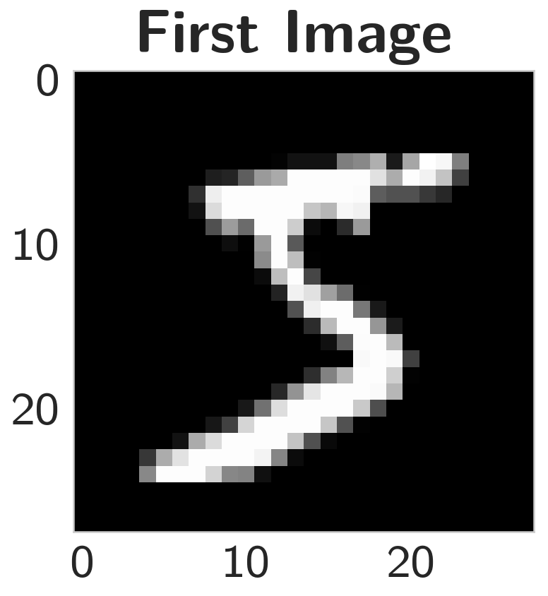
img = numpy.squeeze(images[0])

Plot

figure, axe = pyplot.subplots()
figure.suptitle("First Image", weight="bold")
image = axe.imshow(img, cmap='gray')
first_image.png

Convolutional Autoencoder

Encoder

The encoder part of the network will be a typical convolutional pyramid. Each convolutional layer will be followed by a max-pooling layer to reduce the dimensions of the layers.

Decoder

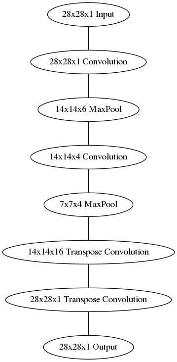
The decoder, though, might be something new to you. The decoder needs to convert from a narrow representation to a wide, reconstructed image. For example, the representation could be a 7x7x4 max-pool layer. This is the output of the encoder, but also the input to the decoder. We want to get a 28x28x1 image out from the decoder so we need to work our way back up from the compressed representation. A schematic of the network is shown below.

graph = Graph(format="png")

# Input layer
graph.node("a", "28x28x1 Input")

# the Encoder
graph.node("b", "28x28x16 Convolution")
graph.node("c", "14x14x16 MaxPool")
graph.node("d", "14x14x4 Convolution")
graph.node("e", "7x7x4 MaxPool")

# The Decoder
graph.node("f", "14x14x16 Transpose Convolution")
graph.node("g", "28x28x1 Transpose Convolution")

# The Output
graph.node("h", "28x28x1 Output")

edges = "abcdefgh"
graph.edges([edges[edge] + edges[edge+1] for edge in range(len(edges) - 1)])

graph.render("graphs/network_graph.dot")
graph

# Out[12]: network_graph.dot.png

:END:

network_graph.dot.png

Here our final encoder layer has size 7x7x4 = 196. The original images have size 28x28 = 784, so the encoded vector is 25% the size of the original image. These are just suggested sizes for each of the layers. Feel free to change the depths and sizes, in fact, you're encouraged to add additional layers to make this representation even smaller! Remember our goal here is to find a small representation of the input data.

Transpose Convolutions, Decoder

This decoder uses transposed convolutional layers to increase the width and height of the input layers. They work almost exactly the same as convolutional layers, but in reverse. A stride in the input layer results in a larger stride in the transposed convolution layer. For example, if you have a 3x3 kernel, a 3x3 patch in the input layer will be reduced to one unit in a convolutional layer. Comparatively, one unit in the input layer will be expanded to a 3x3 path in a transposed convolution layer. PyTorch provides us with an easy way to create the layers, nn.ConvTranspose2d.

It is important to note that transpose convolution layers can lead to artifacts in the final images, such as checkerboard patterns. This is due to overlap in the kernels which can be avoided by setting the stride and kernel size equal. In this Distill article from Augustus Odena, et al, the authors show that these checkerboard artifacts can be avoided by resizing the layers using nearest neighbor or bilinear interpolation (upsampling) followed by a convolutional layer.

We'll show this approach in another notebook, so you can experiment with it and see the difference.

  • Build the encoder out of a series of convolutional and pooling layers.
  • When building the decoder, recall that transpose convolutional layers can upsample an input by a factor of 2 using a stride and kernel_size of 2.

See:

To get the output size of our Convolutional Layers you use the formula:

\[ o = \frac{W - F + 2P}{S} + 1 \]

Where W is the input size (28 here), F is the filter size, P is the zero-padding, and S is the stride. For our first layer we want to keep the output the same size as the input.

The output for a maxpool layer uses a similar set of equations.

\begin{align} W_2 &= \frac{W_1 - F}{S} + 1\\ H_2 &= \frac{H_Y - F}{S} + 1\\ D_2 = D_1\\ \end{align}

Where W is the width, H is the height, and D is the depth.

Layer = namedtuple("Layer", "kernel stride depth padding".split())
Layer.__new__.__defaults__= (0,)
def output_size(input_size: int, layer: Layer, expected: int) -> int:
    """Calculates the output size of the layer

    Args:
     input_size: the size of the input to the layer
     layer: named tuple with values for the layer
     expected: the value you are expecting

    Returns:
     the size of the output

    Raises:
     AssertionError: the calculated value wasn't the expected one
    """
    size = 1 + ((input_size - layer.kernel + 2 * layer.padding)/layer.stride)
    print(layer)
    print("Layer Output Size: {}".format(size))
    assert size == expected
    return size

The Encoder Layers

Layer One

The first layer is a Convolutional Layer that we want to have the same size output as the input but with a depth of sixteen. The CS 231 page notes that to keep the size of the output the same as the input you should set the stride to one and once you have decided on your kernle size (F) then you can find your padding using this equation:

\[ P = \frac{F - 1}{2} \]

In this case I'm going to use a filter size of three so our padding will be:

\begin{align} P &= \frac{3 - 1}{2}\\ &= 1\\ \end{align}

We can double-check this by plugging the values back intoo the equation for output size.

\begin{align} W' &= \frac{W - F + 2P}{S} + 1\\ &= \frac{28 - 3 + 2(1)}{1} + 1\\ &= 28\\ \end{align}
Variable Description
W One dimension of the input
F One dimension of the Kernel (filter)
S Stride
 layer_one = Layer(kernel = 3,
                   padding = 1,
                   stride = 1,
                   depth = 16)

 INPUT_ONE = 28
 OUTPUT_ONE = output_size(INPUT_ONE, layer_one, INPUT_ONE)
 INPUT_DEPTH = 1
Layer(kernel=3, stride=1, depth=16, padding=1)
Layer Output Size: 28.0

Layer Two

The second layer is a MaxPool layer that will keep the depth of six but will halve the size to fourteen. According to the CS 231 n page on Convolutional Networks, there are only two values for the kernel size that are usually used - 2 and 3, and the stride is usually just 2, with a kernel size of 2 being more common, and as it turns out, a kernel size of 2 and a stride of 2 will reduce our input dimensions by a half, which is what we want.

\begin{align} W &= \frac{28 - 2}{2} + 1\\ &= 14\\ \end{align}
 layer_two = Layer(kernel=2, stride=2, depth=layer_one.depth)
 OUTPUT_TWO = output_size(OUTPUT_ONE, layer_two, 14)
Layer(kernel=2, stride=2, depth=16, padding=0)
Layer Output Size: 14.0

Layer Three

Our third layer is another convolutional layer that preserves the input width and height but this time the output will have a depth of 4.

layer_three = Layer(kernel=3, stride=1, depth=4, padding=1)
OUTPUT_THREE = output_size(OUTPUT_TWO, layer_three, OUTPUT_TWO)
Layer(kernel=3, stride=1, depth=4, padding=1)
Layer Output Size: 14.0

Layer Four

The last layer in the encoder is a max pool layer that reduces the previous layer by half (to dimensions of 7) while preserving the depth.

layer_four = Layer(kernel=2, stride=2, depth=layer_three.depth)
OUTPUT_FOUR = output_size(OUTPUT_THREE, layer_four, 7)
Layer(kernel=2, stride=2, depth=4, padding=0)
Layer Output Size: 7.0

Decoders

Layer Five

We want an output of 14 x 14 x 16 from an input of 7 x 7 x 4. The comments given with this exercise say that using a kernel of 2 and stride of 2 will double the dimensions, much as those same values halve the dimensions with Max-Pooling.

layer_five = Layer(kernel=2, stride=2, depth=16)

Layer Six

This layer will expand the image back to its original size of 28 x 28 x 1

layer_six = Layer(kernel=2, stride=2, depth=1)

Define the NN Architecture

class ConvAutoencoder(nn.Module):
    """A CNN AutoEncoder-Decoder"""
    def __init__(self) -> None:
        super().__init__()
        ## encoder layers ##
        self.convolution_1 = nn.Conv2d(in_channels=INPUT_DEPTH,
                                       out_channels=layer_one.depth,
                                       kernel_size=layer_one.kernel, 
                                       stride=layer_one.stride,
                                       padding=layer_one.padding)

        self.max_pool = nn.MaxPool2d(kernel_size=layer_two.kernel,
                                       stride=layer_two.stride)

        self.convolution_2 = nn.Conv2d(in_channels=layer_two.depth,
                                       out_channels=layer_three.depth,
                                       kernel_size=layer_three.kernel,
                                       stride=layer_three.stride,
                                       padding=layer_three.padding)

        ## decoder layers ##
        self.transpose_convolution_1 = nn.ConvTranspose2d(
            in_channels=layer_four.depth, 
            out_channels=layer_five.depth,
            kernel_size=layer_five.kernel,
            stride=layer_five.kernel)

        self.transpose_convolution_2 = nn.ConvTranspose2d(
            in_channels=layer_five.depth, 
            out_channels=layer_six.depth,
            kernel_size=layer_six.kernel,
            stride=layer_six.kernel)

        self.relu = nn.ReLU()
        self.sigmoid = nn.Sigmoid()
        return

    def forward(self, x: torch.Tensor):
        ## encode ##
        x = self.max_pool(self.relu(self.convolution_1(x)))
        x = self.max_pool(self.relu(self.convolution_2(x)))
        ## decode ##
        x = self.relu(self.transpose_convolution_1(x))
        return self.sigmoid(self.transpose_convolution_2(x))
test = ConvAutoencoder()
dataiter = iter(train_loader)
images, labels = dataiter.next()
x = test.convolution_1(images)
print(x.shape)
assert x.shape == torch.Size([BATCH_SIZE, 16, 28, 28])
x = test.max_pool_1(x)
print(x.shape)
assert x.shape == torch.Size([BATCH_SIZE, 16, 14, 14])
x = test.relu(x)
print(x.shape)
assert x.shape == torch.Size([BATCH_SIZE, 16, 14, 14])

x = test.convolution_2(x)
print(x.shape)
assert x.shape == torch.Size([BATCH_SIZE, 4, 14, 14])

x = test.max_pool_2(x)
print(x.shape)
assert x.shape == torch.Size([BATCH_SIZE, 4, 7, 7])

x = test.relu(x)
print(x.shape)
assert x.shape == torch.Size([BATCH_SIZE, 4, 7, 7])

x = test.transpose_convolution_1(x)
print(x.shape)
assert x.shape == torch.Size([BATCH_SIZE, 16, 14, 14])

x = test.relu(x)
print(x.shape)
assert x.shape == torch.Size([BATCH_SIZE, 16, 14, 14])

x = test.transpose_convolution_2(x)
print(x.shape)
assert x.shape == torch.Size([BATCH_SIZE, 1, 28, 28])
torch.Size([20, 16, 28, 28])
torch.Size([20, 16, 14, 14])
torch.Size([20, 4, 14, 14])
torch.Size([20, 4, 7, 7])
torch.Size([20, 16, 14, 14])
torch.Size([20, 1, 28, 28])

Initialize The NN

model = ConvAutoencoder()
print(model)
model.to(device)
ConvAutoencoder(
  (convolution_1): Conv2d(1, 16, kernel_size=(3, 3), stride=(1, 1), padding=(1, 1))
  (max_pool): MaxPool2d(kernel_size=2, stride=2, padding=0, dilation=1, ceil_mode=False)
  (convolution_2): Conv2d(16, 4, kernel_size=(3, 3), stride=(1, 1), padding=(1, 1))
  (transpose_convolution_1): ConvTranspose2d(4, 16, kernel_size=(2, 2), stride=(2, 2))
  (transpose_convolution_2): ConvTranspose2d(16, 1, kernel_size=(2, 2), stride=(2, 2))
  (relu): ReLU()
  (sigmoid): Sigmoid()
)

Training

Here I'll write a bit of code to train the network. I'm not too interested in validation here, so I'll just monitor the training loss and the test loss afterwards.

We are not concerned with labels in this case, just images, which we can get from the train_loader. Because we're comparing pixel values in input and output images, it will be best to use a loss that is meant for a regression task. Regression is all about comparing quantities rather than probabilistic values. So, in this case, I'll use MSELoss. And compare output images and input images as follows:

loss = criterion(outputs, images)

Otherwise, this is pretty straightfoward training with PyTorch. Since this is a convolutional autoencoder, our images do not need to be flattened before being passed in an input to our model.

Train the Model

criterion = nn.MSELoss()
optimizer = torch.optim.Adam(model.parameters(), lr=0.001)
n_epochs = 30
started = datetime.now()
model.train()
for epoch in range(1, n_epochs+1):
    # monitor training loss
    train_loss = 0.0

    ###################
    # train the model #
    ###################

    for data in train_loader:
        # _ stands in for labels, here
        # no need to flatten images
        images, _ = data
        images = images.to(device)
        # clear the gradients of all optimized variables
        optimizer.zero_grad()
        # forward pass: compute predicted outputs by passing inputs to the model
        outputs = model(images)
        # calculate the loss
        loss = criterion(outputs, images)
        # backward pass: compute gradient of the loss with respect to model parameters
        loss.backward()
        # perform a single optimization step (parameter update)
        optimizer.step()
        # update running training loss
        train_loss += loss.item()*images.size(0)

    # print avg training statistics 
    train_loss = train_loss/len(train_loader)
    print('Epoch: {} \tTraining Loss: {:.6f}'.format(
        epoch, 
        train_loss
        ))
ended = datetime.now()
print("Ended: {}".format(ended))
print("Elapsed: {}".format(ended - started))
Epoch: 1        Training Loss: 0.259976
Epoch: 2        Training Loss: 0.244956
Epoch: 3        Training Loss: 0.235354
Epoch: 4        Training Loss: 0.226544
Epoch: 5        Training Loss: 0.216255
Epoch: 6        Training Loss: 0.207204
Epoch: 7        Training Loss: 0.200490
Epoch: 8        Training Loss: 0.195582
Epoch: 9        Training Loss: 0.191870
Epoch: 10       Training Loss: 0.189247
Epoch: 11       Training Loss: 0.187027
Epoch: 12       Training Loss: 0.185084
Epoch: 13       Training Loss: 0.183055
Epoch: 14       Training Loss: 0.181224
Epoch: 15       Training Loss: 0.179749
Epoch: 16       Training Loss: 0.178564
Epoch: 17       Training Loss: 0.177572
Epoch: 18       Training Loss: 0.176735
Epoch: 19       Training Loss: 0.176076
Epoch: 20       Training Loss: 0.175518
Epoch: 21       Training Loss: 0.175040
Epoch: 22       Training Loss: 0.174629
Epoch: 23       Training Loss: 0.174230
Epoch: 24       Training Loss: 0.173856
Epoch: 25       Training Loss: 0.173497
Epoch: 26       Training Loss: 0.173166
Epoch: 27       Training Loss: 0.172838
Epoch: 28       Training Loss: 0.172520
Epoch: 29       Training Loss: 0.172212
Epoch: 30       Training Loss: 0.171920
Ended: 2018-12-21 17:41:26.461977
Elapsed: 0:07:50.942721

Checking out the results

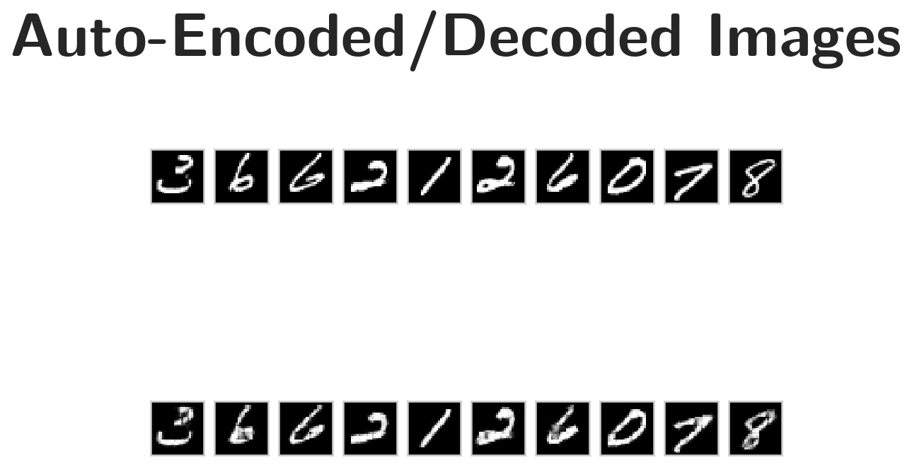
Below I've plotted some of the test images along with their reconstructions. These look a little rough around the edges, likely due to the checkerboard effect we mentioned above that tends to happen with transpose layers.

Obtain One Batch Of Test Images

dataiter = iter(test_loader)
images, labels = dataiter.next()
images = images.to(device)

Get Sample Outputs

output = model(images)

Prep Images for Display

images = images.cpu().numpy()

Output Is Resized Into a Batch Of Images

output = output.view(BATCH_SIZE, 1, 28, 28)

Use Detach When It's An Output That Requires Grad

output = output.detach().cpu().numpy()

plot the first ten input images and then reconstructed images

figure, axes = pyplot.subplots(nrows=2, ncols=10, sharex=True, sharey=True)
figure.suptitle("Auto-Encoded/Decoded Images", weight="bold")
# input images on top row, reconstructions on bottom
for images, row in zip([images, output], axes):
    for img, ax in zip(images, row):
        ax.imshow(numpy.squeeze(img), cmap='gray')
        ax.get_xaxis().set_visible(False)
        ax.get_yaxis().set_visible(False)
reconstructed.png

That is better than I would have thought it would be.

Simple Autoencoder

Introduction

We'll start off by building a simple autoencoder to compress the MNIST dataset. With autoencoders, we pass input data through an encoder that makes a compressed representation of the input. Then, this representation is passed through a decoder to reconstruct the input data. Generally the encoder and decoder will be built with neural networks, then trained on example data.

Compressed Representation

A compressed representation can be great for saving and sharing any kind of data in a way that is more efficient than storing raw data. In practice, the compressed representation often holds key information about an input image and we can use it for denoising images or other kinds of reconstruction and transformation!

Set Up

In this notebook, we'll be build a simple network architecture for the encoder and decoder. Let's get started by importing our libraries and getting the dataset.

Imports

PyPi

from dotenv import load_dotenv
from torchvision import datasets
import matplotlib.pyplot as pyplot
import numpy
import seaborn
import torch
import torch.nn as nn
import torch.nn.functional as F
import torchvision.transforms as transforms

This Project

from neurotic.tangles.data_paths import DataPathTwo

Plotting

get_ipython().run_line_magic('matplotlib', 'inline')
get_ipython().run_line_magic('config', "InlineBackend.figure_format = 'retina'")
seaborn.set(style="whitegrid",
            rc={"axes.grid": False,
                "font.family": ["sans-serif"],
                "font.sans-serif": ["Open Sans", "Latin Modern Sans", "Lato"],
                "figure.figsize": (8, 6)},
            font_scale=3)

The Data

Data Transformer

transform = transforms.ToTensor()

Load the Data

load_dotenv()
path = DataPathTwo(folder_key="MNIST")
print(path.folder)
/home/hades/datasets/MNIST
train_data = datasets.MNIST(root=path.folder, train=True,
                            download=True, transform=transform)
test_data = datasets.MNIST(root=path.folder, train=False,
                           download=True, transform=transform)

Training and Test Batch Loaders

  • Some Constants
    # number of subprocesses to use for data loading
    NUM_WORKERS = 0
    # how many samples per batch to load
    BATCH_SIZE = 20
    

    Prepare the loaders.

    train_loader = torch.utils.data.DataLoader(train_data,
                                               batch_size=BATCH_SIZE,
                                               num_workers=NUM_WORKERS)
    test_loader = torch.utils.data.DataLoader(test_data,
                                              batch_size=BATCH_SIZE,
                                              num_workers=NUM_WORKERS)
    

Visualize the Data

Obtain One Batch of Training Images

dataiter = iter(train_loader)
images, labels = dataiter.next()
images = images.numpy()

Get One Image From the Batch

img = numpy.squeeze(images[0])
figure, axe = pyplot.subplots()
figure.suptitle("First Image", weight="bold")
image = axe.imshow(img, cmap='gray')

first_image.png

Linear Autoencoder

Description

We'll train an autoencoder with these images by flattening them into 784 length vectors. The images from this dataset are already normalized such that the values are between 0 and 1. Let's start by building a simple autoencoder. The encoder and decoder should be made of one linear layer. The units that connect the encoder and decoder will be the compressed representation.

Since the images are normalized between 0 and 1, we need to use a sigmoid activation on the output layer to get values that match this input value range.

  • The input images will be flattened into 784 length vectors. The targets are the same as the inputs.
  • The encoder and decoder will be made of two linear layers, each.
  • The depth dimensions should change as follows: 784 inputs > encoding_dim > 784 outputs.
  • All layers will have ReLu activations applied except for the final output layer, which has a sigmoid activation.

The compressed representation should be a vector with dimension encoding_dim=32.

Architecture Definition

rows, columns = img.shape
IMAGE_DIMENSION = rows * columns
class Autoencoder(nn.Module):
    """"" simple autoencoder-decoder

    Args:
     encoding_dim: the dimension of the encoded image
    """
    def __init__(self, encoding_dim:int):
        super().__init__()
        self.encoder = nn.Linear(IMAGE_DIMENSION, encoding_dim)
        self.activation_one = nn.ReLU()
        self.decoder = nn.Linear(encoding_dim, IMAGE_DIMENSION)
        self.activation_output = nn.Sigmoid()
        return


    def forward(self, x: torch.Tensor) -> torch.Tensor:
        """Does one feed-forward pass

       Args:
        x: flattened MNIST image

       Returns:
        the encoded-decoded version of the image
       """
        x = self.activation_one(self.encoder(x))
        return self.activation_output(self.decoder(x))

Initialize the Auto-Encoder

encoding_dim = 32
model = Autoencoder(encoding_dim)
print(model)
Autoencoder(
  (encoder): Linear(in_features=784, out_features=32, bias=True)
  (activation_one): ReLU()
  (decoder): Linear(in_features=32, out_features=784, bias=True)
  (activation_output): Sigmoid()
)

Training

Here I'll write a bit of code to train the network. I'm not too interested in validation here, so I'll just monitor the training loss and the test loss afterwards.

We are not concerned with labels in this case, just images, which we can get from the train_loader. Because we're comparing pixel values in input and output images, it will be best to use a loss that is meant for a regression task. Regression is all about comparing quantities rather than probabilistic values. So, in this case, I'll use MSELoss, which calculates the Mean-Squared Error between the predicted and the actual value, and compare output images and input images as follows:

loss = criterion(outputs, images)

Otherwise, this is pretty straightfoward training with PyTorch. We flatten our images, pass them into the autoencoder, and record the training loss as we go.

Specify the Loss Function

criterion = nn.MSELoss()

Specifiy the Optimizer

We're going to use the Adam optimizer instead of Stochastic Gradient Descent.

optimizer = torch.optim.Adam(model.parameters(), lr=0.001)

And Now We Train

n_epochs = 20

for epoch in range(1, n_epochs+1):
    # monitor training loss
    train_loss = 0.0

    ###################
    # train the model #
    ###################
    for data in train_loader:
        # _ stands in for labels, here
        images, _ = data
        # flatten images
        images = images.view(images.size(0), -1)
        # clear the gradients of all optimized variables
        optimizer.zero_grad()
        # forward pass: compute predicted outputs by passing inputs to the model
        outputs = model(images)
        # calculate the loss
        loss = criterion(outputs, images)
        # backward pass: compute gradient of the loss with respect to model parameters
        loss.backward()
        # perform a single optimization step (parameter update)
        optimizer.step()
        # update running training loss
        train_loss += loss.item()*images.size(0)

    # print avg training statistics 
    train_loss = train_loss/len(train_loader)
    print('Epoch: {} \tTraining Loss: {:.6f}'.format(
        epoch, 
        train_loss
        ))
Epoch: 1        Training Loss: 0.622334
Epoch: 2        Training Loss: 0.297601
Epoch: 3        Training Loss: 0.258895
Epoch: 4        Training Loss: 0.250710
Epoch: 5        Training Loss: 0.247124
Epoch: 6        Training Loss: 0.244808
Epoch: 7        Training Loss: 0.243222
Epoch: 8        Training Loss: 0.242119
Epoch: 9        Training Loss: 0.241254
Epoch: 10       Training Loss: 0.240563
Epoch: 11       Training Loss: 0.239997
Epoch: 12       Training Loss: 0.239529
Epoch: 13       Training Loss: 0.239120
Epoch: 14       Training Loss: 0.238747
Epoch: 15       Training Loss: 0.238395
Epoch: 16       Training Loss: 0.238030
Epoch: 17       Training Loss: 0.237546
Epoch: 18       Training Loss: 0.237213
Epoch: 19       Training Loss: 0.236916
Epoch: 20       Training Loss: 0.236473

Checking out the results

Below I've plotted some of the test images along with their reconstructions. For the most part these look pretty good except for some blurriness in some parts.

Obtain One Batch Of Test Images

dataiter = iter(test_loader)
images, labels = dataiter.next()

images_flatten = images.view(images.size(0), -1)

# get sample outputs
output = model(images_flatten)
# prep images for display
images = images.numpy()


# output is resized into a batch of images
output = output.view(BATCH_SIZE, 1, 28, 28)
# use detach when it's an output that requires_grad
output = output.detach().numpy()
figure, axes = pyplot.subplots(nrows=2, ncols=10, sharex=True, sharey=True, figsize=(10,8))

# input images on top row, reconstructions on bottom
for images, row in zip([images, output], axes):
    for img, ax in zip(images, row):
        ax.imshow(numpy.squeeze(img), cmap='gray')
        ax.get_xaxis().set_visible(False)
        ax.get_yaxis().set_visible(False)

recomposed.png

Weight Initialization

Introduction

In this lesson, you'll learn how to find good initial weights for a neural network. Weight initialization happens once, when a model is created and before it trains. Having good initial weights can place the neural network close to the optimal solution. This allows the neural network to come to the best solution quicker.

Initial Weights and Observing Training Loss

To see how different weights perform, we'll test on the same dataset and neural network. That way, we know that any changes in model behavior are due to the weights and not any changing data or model structure. We'll instantiate at least two of the same models, with different initial weights and see how the training loss decreases over time.

Sometimes the differences in training loss, over time, will be large and other times, certain weights offer only small improvements.

Dataset and Model

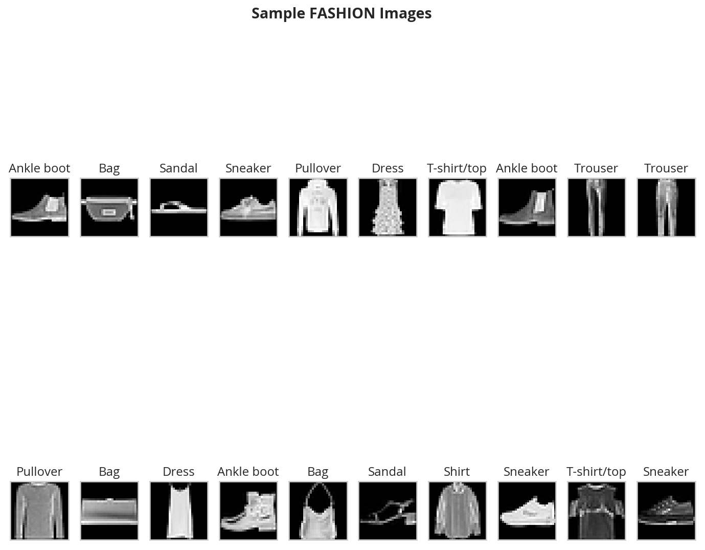
We'll train an MLP to classify images from the Fashion-MNIST database to demonstrate the effect of different initial weights. As a reminder, the FashionMNIST dataset contains images of clothing types; classes = ['T-shirt/top', 'Trouser', 'Pullover', 'Dress', 'Coat', 'Sandal', 'Shirt', 'Sneaker', 'Bag', 'Ankle boot']. The images are normalized so that their pixel values are in a range [0.0 - 1.0). Run the cell below to download and load the dataset.

Import Libraries and Load the Data

Imports

# python
from functools import partial
from typing import Collection, Tuple
# from pypi
from dotenv import load_dotenv
from sklearn.model_selection import train_test_split
from torch.utils.data.sampler import SubsetRandomSampler
from torchvision import datasets
import matplotlib.pyplot as pyplot
import numpy
import seaborn
import torch
import torch.nn as nn
import torch.nn.functional as F
import torchvision.transforms as transforms

# udacity
import nano.helpers as helpers

# this project
from neurotic.tangles.data_paths import DataPathTwo

Load the Data

# number of subprocesses to use for data loading
subprocesses = 0
# how many samples per batch to load
batch_size = 100
# percentage of training set to use as validation
VALIDATION_FRACTION = 0.2

Convert the data to a torch.FloatTensor.

transform = transforms.ToTensor()
load_dotenv()
path = DataPathTwo(folder_key="FASHION")
print(path.folder)
/home/brunhilde/datasets/FASHION

Choose the training and test datasets.

train_data = datasets.FashionMNIST(root=path.folder, train=True,
                                   download=True, transform=transform)
test_data = datasets.FashionMNIST(root=path.folder, train=False,
                                  download=True, transform=transform)
Downloading http://fashion-mnist.s3-website.eu-central-1.amazonaws.com/train-images-idx3-ubyte.gz
Downloading http://fashion-mnist.s3-website.eu-central-1.amazonaws.com/train-labels-idx1-ubyte.gz
Downloading http://fashion-mnist.s3-website.eu-central-1.amazonaws.com/t10k-images-idx3-ubyte.gz
Downloading http://fashion-mnist.s3-website.eu-central-1.amazonaws.com/t10k-labels-idx1-ubyte.gz
Processing...
Done!

Obtain training indices that will be used for validation.

indices = list(range(len(train_data)))
train_idx, valid_idx = train_test_split(
    indices,
    test_size=VALIDATION_FRACTION)

Define samplers for obtaining training and validation batches.

train_sampler = SubsetRandomSampler(train_idx)
valid_sampler = SubsetRandomSampler(valid_idx)

Prepare data loaders (combine dataset and sampler).

train_loader = torch.utils.data.DataLoader(train_data, batch_size=batch_size,
                                           sampler=train_sampler, num_workers=subprocesses)
valid_loader = torch.utils.data.DataLoader(train_data, batch_size=batch_size, 
                                           sampler=valid_sampler, num_workers=subprocesses)
test_loader = torch.utils.data.DataLoader(test_data, batch_size=batch_size, 
                                          num_workers=subprocesses)
classes = ['T-shirt/top', 'Trouser', 'Pullover', 'Dress', 'Coat', 
    'Sandal', 'Shirt', 'Sneaker', 'Bag', 'Ankle boot']

Visualize Some Training Data

get_ipython().run_line_magic('matplotlib', 'inline')
get_ipython().run_line_magic('config', "InlineBackend.figure_format = 'retina'")
seaborn.set(style="whitegrid",
            rc={"axes.grid": False,
                "font.family": ["sans-serif"],
                "font.sans-serif": ["Open Sans", "Latin Modern Sans", "Lato"],
                "figure.figsize": (10, 8)},
            font_scale=1)

Obtain one batch of training images.

dataiter = iter(train_loader)
images, labels = dataiter.next()
images = images.numpy()

Plot the images in the batch, along with the corresponding labels.

fig = pyplot.figure(figsize=(12, 10))
fig.suptitle("Sample FASHION Images", weight="bold")
for idx in np.arange(20):
    ax = fig.add_subplot(2, 20/2, idx+1, xticks=[], yticks=[])
    ax.imshow(np.squeeze(images[idx]), cmap='gray')
    ax.set_title(classes[labels[idx]])

image_one.png

Define the Model Architecture

We've defined the MLP that we'll use for classifying the dataset.

Neural Network

  • A 3 layer MLP with hidden dimensions of 256 and 128.
  • This MLP accepts a flattened image (784-value long vector) as input and produces 10 class scores as output.

We'll test the effect of different initial weights on this 3 layer neural network with ReLU activations and an Adam optimizer. The lessons you learn apply to other neural networks, including different activations and optimizers.

Initialize Weights

Let's start looking at some initial weights.

All Zeros or Ones

If you follow the principle of Occam's razor, you might think setting all the weights to 0 or 1 would be the best solution. This is not the case.

With every weight the same, all the neurons at each layer are producing the same output. This makes it hard to decide which weights to adjust.

Let's compare the loss with all ones and all zero weights by defining two models with those constant weights.

Below, we are using PyTorch's nn.init to initialize each Linear layer with a constant weight. The init library provides a number of weight initialization functions that give you the ability to initialize the weights of each layer according to layer type.

In the case below, we look at every layer/module in our model. If it is a Linear layer (as all three layers are for this MLP), then we initialize those layer weights to be a constant_weight with bias=0 using the following code:

if isinstance(m, nn.Linear):
    nn.init.constant_(m.weight, constant_weight)
    nn.init.constant_(m.bias, 0)

The constant_weight is a value that you can pass in when you instantiate the model.

Define the NN architecture

class Net(nn.Module):
    def __init__(self, hidden_1=256, hidden_2=128, constant_weight=None):
        super(Net, self).__init__()
        # linear layer (784 -> hidden_1)
        self.fc1 = nn.Linear(28 * 28, hidden_1)
        # linear layer (hidden_1 -> hidden_2)
        self.fc2 = nn.Linear(hidden_1, hidden_2)
        # linear layer (hidden_2 -> 10)
        self.fc3 = nn.Linear(hidden_2, 10)
        # dropout layer (p=0.2)
        self.dropout = nn.Dropout(0.2)

        # initialize the weights to a specified, constant value
        if(constant_weight is not None):
            for m in self.modules():
                if isinstance(m, nn.Linear):
                    nn.init.constant_(m.weight, constant_weight)
                    nn.init.constant_(m.bias, 0)


    def forward(self, x):
        # flatten image input
        x = x.view(-1, 28 * 28)
        # add hidden layer, with relu activation function
        x = F.relu(self.fc1(x))
        # add dropout layer
        x = self.dropout(x)
        # add hidden layer, with relu activation function
        x = F.relu(self.fc2(x))
        # add dropout layer
        x = self.dropout(x)
        # add output layer
        x = self.fc3(x)
        return x

Compare Model Behavior

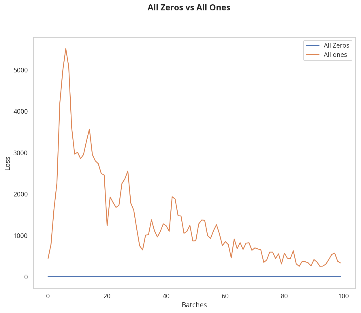
Below, we are using helpers.compare_init_weights to compare the training and validation loss for the two models we defined above, model_0 and model_1. This function takes in a list of models (each with different initial weights), the name of the plot to produce, and the training and validation dataset loaders. For each given model, it will plot the training loss for the first 100 batches and print out the validation accuracy after 2 training epochs. Note: if you've used a small batch_size, you may want to increase the number of epochs here to better compare how models behave after seeing a few hundred images.

We plot the loss over the first 100 batches to better judge which model weights performed better at the start of training. I recommend that you take a look at the code in helpers.py to look at the details behind how the models are trained, validated, and compared.

Run the cell below to see the difference between weights of all zeros against all ones.

Initialize two NN's with 0 and 1 constant weights.

model_0 = Net(constant_weight=0)
model_1 = Net(constant_weight=1)

Put them in list form to compare.

model_list = [(model_0, 'All Zeros'),
              (model_1, 'All Ones')]
ModelLabel = Tuple[nn.Module, str]
ModelLabels = Collection[ModelLabel]
def plot_models(title:str, models_labels:ModelLabels):
    """Plots the models

    Args:
     title: the title for the plots
     models_labels: collections of model, plot-label tuples
    """
    figure, axe = pyplot.subplots()
    figure.suptitle(title, weight="bold")    
    axe.set_xlabel("Batches")
    axe.set_ylabel("Loss")

    for model, label in models_labels:
        loss, validation_accuracy = helpers._get_loss_acc(model, train_loader, valid_loader)
        axe.plot(loss[:100], label=label)
    legend = axe.legend()
    return

Plot the loss over the first 100 batches.

plot_models("All Zeros vs All Ones",
            ((model_0, "All Zeros"),
             (model_1, "All ones")))

zeros_ones.png

After 2 Epochs:
Validation Accuracy
    9.475% -- All Zeros
   10.175% -- All Ones
Training Loss
    2.304  -- All Zeros
  1914.703  -- All Ones

As you can see the accuracy is close to guessing for both zeros and ones, around 10%.

The neural network is having a hard time determining which weights need to be changed, since the neurons have the same output for each layer. To avoid neurons with the same output, let's use unique weights. We can also randomly select these weights to avoid being stuck in a local minimum for each run.

A good solution for getting these random weights is to sample from a uniform distribution.

Uniform Distribution

A uniform distribution has the equal probability of picking any number from a set of numbers. We'll be picking from a continuous distribution, so the chance of picking the same number is low. We'll use NumPy's np.random.uniform function to pick random numbers from a uniform distribution.

np.random_uniform(low=0.0, high=1.0, size=None)

Outputs random values from a uniform distribution.

The generated values follow a uniform distribution in the range [low, high). The lower bound minval is included in the range, while the upper bound maxval is excluded.

  • low: The lower bound on the range of random values to generate. Defaults to 0.
  • high: The upper bound on the range of random values to generate. Defaults to 1.
  • size: An int or tuple of ints that specify the shape of the output array.

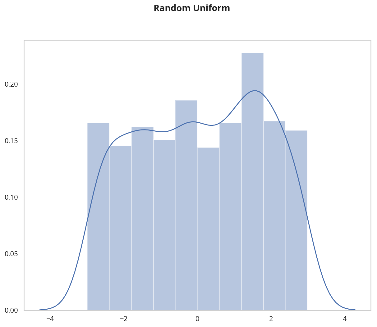
We can visualize the uniform distribution by using a histogram. Let's map the values from np.random_uniform(-3, 3, [1000]) to a histogram using the helper.hist_dist function. This will be 1000 random float values from -3 to 3, excluding the value 3.

figure, axe = pyplot.subplots()
figure.suptitle("Random Uniform", weight="bold")
data = numpy.random.uniform(-3, 3, [1000])
grid = seaborn.distplot(data)
#helpers.hist_dist('Random Uniform (low=-3, high=3)', )

uniform_distribution.png

Now that you understand the uniform function, let's use PyTorch's nn.init to apply it to a model's initial weights.

Uniform Initialization, Baseline

Let's see how well the neural network trains using a uniform weight initialization, where low=0.0 and high=1.0. Below, I'll show you another way (besides in the Net class code) to initialize the weights of a network. To define weights outside of the model definition, you can:

  1. Define a function that assigns weights by the type of network layer, then
  2. Apply those weights to an initialized model using model.apply(fn), which applies a function to each model layer.

This time, we'll use weight.data.uniform_ to initialize the weights of our model, directly.

def weights_init_uniform(m: nn.Module, start=0.0, stop=1.0) -> None:
    """takes in a module and applies the specified weight initialization

    Args:
     m: A model instance
    """
    classname = m.__class__.__name__
    # for every Linear layer in a model..
    if classname.startswith('Linear'):
        # apply a uniform distribution to the weights and a bias=0
        m.weight.data.uniform_(start, stop)
        m.bias.data.fill_(0)
    return

Create A New Model With These Weights

Evaluate Behavior

model_uniform = Net()
model_uniform.apply(weights_init_uniform)
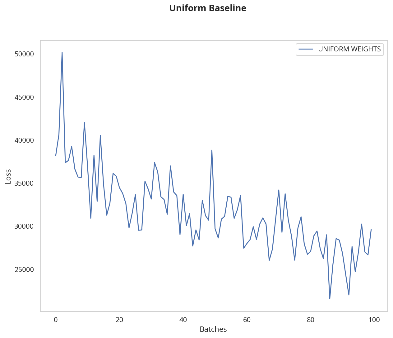
plot_models("Uniform Baseline", ((model_uniform, "UNIFORM WEIGHTS"),))

uniform_weights.png

The loss graph is showing the neural network is learning, which it didn't with all zeros or all ones. We're headed in the right direction!

General rule for setting weights

The general rule for setting the weights in a neural network is to set them to be close to zero without being too small. A good practice is to start your weights in the range of \([-y, y]\) where \(y=1/\sqrt{n}\) (\(n\) is the number of inputs to a given neuron).

Let's see if this holds true; let's create a baseline to compare with and center our uniform range over zero by shifting it over by 0.5. This will give us the range [-0.5, 0.5).

weights_init_uniform_center = partial(weights_init_uniform, -0.5, 0.5)

create a new model with these weights

model_centered = Net()
model_centered.apply(weights_init_uniform_center)

Now let's create a distribution and model that uses the general rule for weight initialization; using the range \([-y, y]\), where \(y=1/\sqrt{n}\) .

And finally, we'll compare the two models.

def weights_init_uniform_rule(m: nn.Module) -> None:
    """takes in a module and applies the specified weight initialization

    Args:
     m: Model instance
    """
    classname = m.__class__.__name__
    # for every Linear layer in a model..
    if classname.find('Linear') != -1:
        # get the number of the inputs
        n = m.in_features
        y = 1.0/numpy.sqrt(n)
        m.weight.data.uniform_(-y, y)
        m.bias.data.fill_(0)
    return
model_rule = Net()
model_rule.apply(weights_init_uniform_rule)
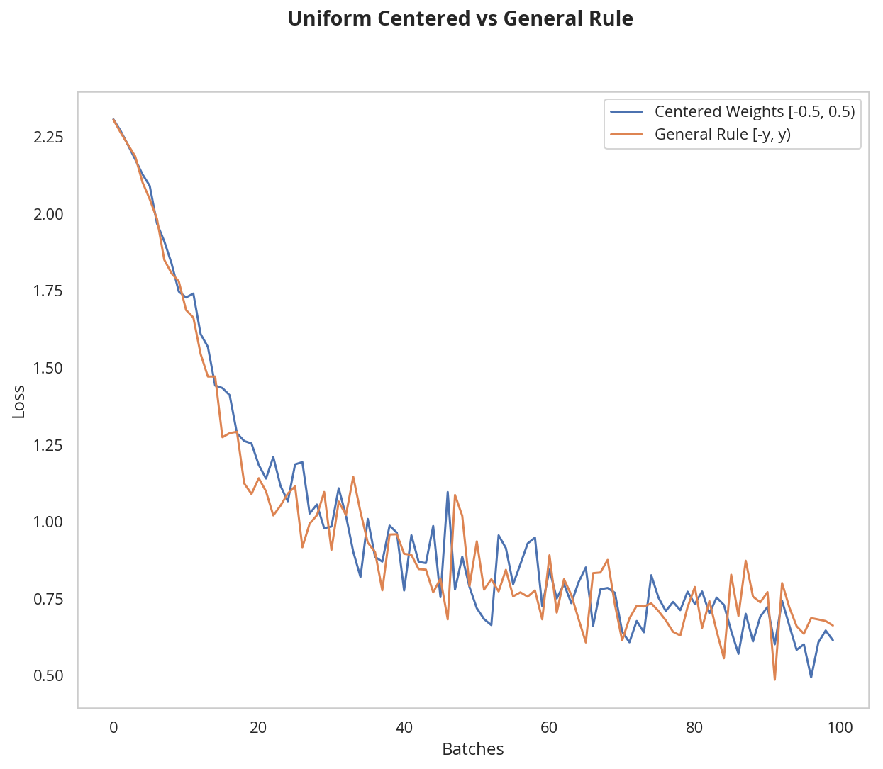
plot_models("Uniform Centered vs General Rule", (
    (model_centered, 'Centered Weights [-0.5, 0.5)'), 
    (model_rule, 'General Rule [-y, y)'),
))

general_rule.png This behavior is really promising! Not only is the loss decreasing, but it seems to do so very quickly for our uniform weights that follow the general rule; after only two epochs we get a fairly high validation accuracy and this should give you some intuition for why starting out with the right initial weights can really help your training process!
Since the uniform distribution has the same chance to pick any value in a range, what if we used a distribution that had a higher chance of picking numbers closer to 0? Let's look at the normal distribution.

Normal Distribution

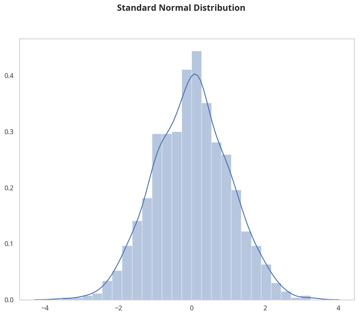
Unlike the uniform distribution, the normal distribution has a higher likelihood of picking number close to it's mean. To visualize it, let's plot values from NumPy's np.random.normal function to a histogram.

np.random.normal(loc=0.0, scale=1.0, size=None)

Outputs random values from a normal distribution.

  • loc: The mean of the normal distribution.
  • scale: The standard deviation of the normal distribution.
  • shape: The shape of the output array.
figure, axe = pyplot.subplots()
figure.suptitle("Standard Normal Distribution", weight="bold")
grid = seaborn.distplot(numpy.random.normal(size=[1000]))

normal_distribution.png

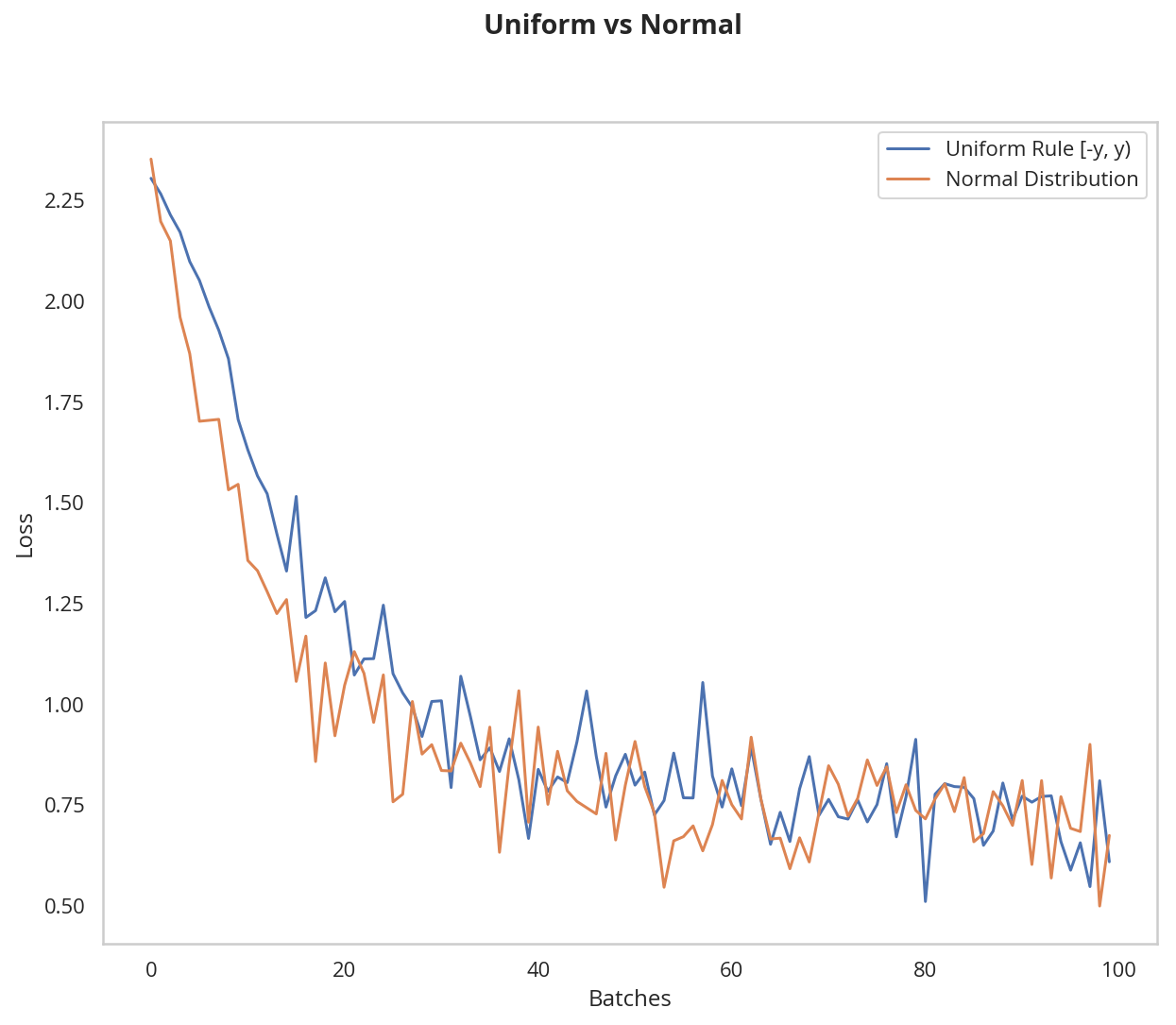
Let's compare the normal distribution against the previous, rule-based, uniform distribution.

The normal distribution should have a mean of 0 and a standard deviation of \(y=1/\sqrt{n}\)

def weights_init_normal(m: nn.Module) -> None:
    '''Takes in a module and initializes all linear layers with weight
       values taken from a normal distribution.'''

    classname = m.__class__.__name__
    if classname.startswith("Linear"):    
        m.weight.data.normal_(mean=0, std=1/numpy.sqrt(m.in_features))
        m.bias.data.fill_(0)
    return

create a new model with the rule-based, uniform weights

model_uniform_rule = Net()
model_uniform_rule.apply(weights_init_uniform_rule)

create a new model with the rule-based, NORMAL weights

model_normal_rule = Net()
model_normal_rule.apply(weights_init_normal)

compare the two models

plot_models('Uniform vs Normal',
            ((model_uniform_rule, 'Uniform Rule [-y, y)'), 
             (model_normal_rule, 'Normal Distribution')))

normal_vs_uniform.png

The normal distribution gives us pretty similar behavior compared to the uniform distribution, in this case. This is likely because our network is so small; a larger neural network will pick more weight values from each of these distributions, magnifying the effect of both initialization styles. In general, a normal distribution will result in better performance for a model.

Automatic Initialization

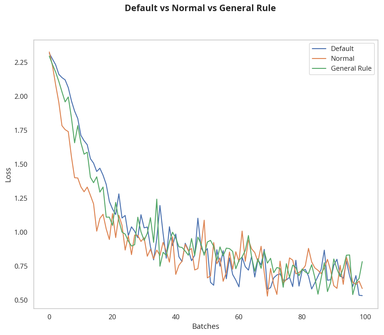
Let's quickly take a look at what happens without any explicit weight initialization.

Instantiate a model with no explicit weight initialization

evaluate the behavior using helpers

model_normal_rule = Net()
model_normal_rule.apply(weights_init_normal)
model_default = Net()
model_rule = Net()
model_rule.apply(weights_init_uniform_rule)

plot_models("Default vs Normal vs General Rule", (
    (model_default, "Default"),
    (model_normal_rule, "Normal"),
    (model_rule, "General Rule")))

default.png

They all sort of look the same at this point.

Transfer Learning Exercise

Introduction

Most of the time you won't want to train a whole convolutional network yourself. Modern ConvNets training on huge datasets like ImageNet take weeks on multiple GPUs. Instead, most people use a pretrained network either as a fixed feature extractor, or as an initial network to fine tune.

In this notebook, you'll be using VGGNet trained on the ImageNet dataset as a feature extractor.

VGGNet is great because it's simple and has great performance, coming in second in the ImageNet competition. The idea here is that we keep all the convolutional layers, but replace the final fully-connected layer with our own classifier. This way we can use VGGNet as a fixed feature extractor for our images then easily train a simple classifier on top of that.

  • Use all but the last fully-connected layer as a fixed feature extractor.
  • Define a new, final classification layer and apply it to a task of our choice!

You can read more about transfer learning from the CS231n Stanford course notes.

Imports

# python
from collections import OrderedDict
from datetime import datetime
import os

# pypi
from dotenv import load_dotenv
from torch import nn
from sklearn.model_selection import train_test_split
from torch.utils.data.sampler import SubsetRandomSampler

import matplotlib
import numpy
import seaborn
import torch
import torch.optim as optimize
import torchvision
from torchvision import datasets, models, transforms
import matplotlib.pyplot as pyplot

# this project
from neurotic.tangles.data_paths import DataPathTwo

Plotting

get_ipython().run_line_magic('matplotlib', 'inline')
get_ipython().run_line_magic('config', "InlineBackend.figure_format = 'retina'")
seaborn.set(style="whitegrid",
            rc={"axes.grid": False,
                "font.size": 8,
                "font.family": ["sans-serif"],
                "font.sans-serif": ["Latin Modern Sans", "Lato"],
                "figure.figsize": (8, 6)},
            font_scale=3)

Flower power

Here we'll be using VGGNet to classify images of flowers. We'll start, as usual, by importing our usual resources. And checking if we can train our model on the GPU.

Download the Data

Download the flower data from this link, save it in the home directory of this notebook and extract the zip file to get the directory flower_photos/. Make sure the directory has this exact name for accessing data: flower_photos.

load_dotenv()
path = DataPathTwo(folder_key="FLOWERS")
print(path.folder)
for target in path.folder.iterdir():
    print(target)
/home/hades/datasets/flower_photos
/home/hades/datasets/flower_photos/.DS_Store
/home/hades/datasets/flower_photos/train
/home/hades/datasets/flower_photos/test
/home/hades/datasets/flower_photos/LICENSE.txt

Check If CUDA Is Available

device = "cuda:0" if torch.cuda.is_available() else "cpu"
print(device)
cuda:0

CUDA is running out of memory and crashing so don't use CUDA.

device = "cpu"
print(device)
cpu

Load and Transform our Data

We'll be using PyTorch's ImageFolder class which makes is very easy to load data from a directory. For example, the training images are all stored in a directory path that looks like this:

root/class_1/xxx.png
root/class_1/xxy.png
root/class_1/xxz.png

root/class_2/123.png
root/class_2/nsdf3.png
root/class_2/asd932_.png

Where, in this case, the root folder for training is flower_photos/train/ and the classes are the names of flower types.

Define Training and Test Data Directories

train_dir = path.folder.joinpath('train/')
test_dir = path.folder.joinpath('test/')
print(train_dir)
print(test_dir)
/home/hades/datasets/flower_photos/train
/home/hades/datasets/flower_photos/test

Classes are folders in each directory with these names:

classes = ['daisy', 'dandelion', 'roses', 'sunflowers', 'tulips']
CLASS_COUNT = len(classes)

Transforming the Data

When we perform transfer learning, we have to shape our input data into the shape that the pre-trained model expects. VGG16 expects `224`-dim square images as input and so, we resize each flower image to fit this mold.

Load And Transform Data Using ImageFolder

VGG-16 Takes 224x224 images as input, so we resize all of them.

data_transform = transforms.Compose([transforms.RandomResizedCrop(224), 
                                      transforms.ToTensor()])

train_data = datasets.ImageFolder(train_dir, transform=data_transform)
test_data = datasets.ImageFolder(test_dir, transform=data_transform)

Print Out Some Data Stats

print('Num training images: ', len(train_data))
print('Num test images: ', len(test_data))
Num training images:  3130
Num test images:  540
VALIDATION_FRACTION = 0.2
indices = list(range(len(train_data)))
training_indices, validation_indices = train_test_split(
    indices,
    test_size=VALIDATION_FRACTION)

DataLoaders and Data Visualization

Define Dataloader Parameters

BATCH_SIZE = 20
NUM_WORKERS=4
train_sampler = SubsetRandomSampler(training_indices)
valid_sampler = SubsetRandomSampler(validation_indices)

Prepare Data Loaders

train_loader = torch.utils.data.DataLoader(train_data, batch_size=BATCH_SIZE, 
                                           sampler=train_sampler,
                                           num_workers=NUM_WORKERS)
valid_loader = torch.utils.data.DataLoader(train_data, batch_size=BATCH_SIZE, 
                                           sampler=valid_sampler, num_workers=NUM_WORKERS)
test_loader = torch.utils.data.DataLoader(test_data, batch_size=batch_size, 
                                          num_workers=num_workers, shuffle=True)

Visualize some sample data

obtain one batch of training images

dataiter = iter(train_loader)
images, labels = dataiter.next()
images = images.numpy() # convert images to numpy for display

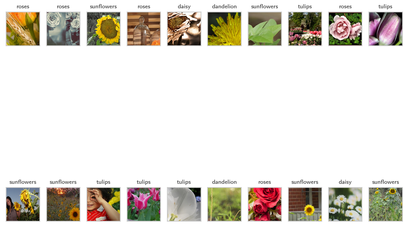
Plot The Images In The Batch, Along With The Corresponding Labels

fig = pyplot.figure(figsize=(12, 10))
pyplot.rc("axes", titlesize=10)
for idx in numpy.arange(20):
    ax = fig.add_subplot(2, 20/2, idx+1, xticks=[], yticks=[])
    pyplot.imshow(numpy.transpose(images[idx], (1, 2, 0)))
    ax.set_title(classes[labels[idx]])

sample_batches.png

Define the Model

To define a model for training we'll follow these steps:

  1. Load in a pre-trained VGG16 model
  2. "Freeze" all the parameters, so the net acts as a fixed feature extractor
  3. Remove the last layer
  4. Replace the last layer with a linear classifier of our own

/Freezing simply means that the parameters in the pre-trained model will not change during training.**

Load the pretrained model from pytorch

vgg16 = models.vgg16(pretrained=True)

Print Out The Model Structure

print(vgg16)
VGG(
  (features): Sequential(
    (0): Conv2d(3, 64, kernel_size=(3, 3), stride=(1, 1), padding=(1, 1))
    (1): ReLU(inplace)
    (2): Conv2d(64, 64, kernel_size=(3, 3), stride=(1, 1), padding=(1, 1))
    (3): ReLU(inplace)
    (4): MaxPool2d(kernel_size=2, stride=2, padding=0, dilation=1, ceil_mode=False)
    (5): Conv2d(64, 128, kernel_size=(3, 3), stride=(1, 1), padding=(1, 1))
    (6): ReLU(inplace)
    (7): Conv2d(128, 128, kernel_size=(3, 3), stride=(1, 1), padding=(1, 1))
    (8): ReLU(inplace)
    (9): MaxPool2d(kernel_size=2, stride=2, padding=0, dilation=1, ceil_mode=False)
    (10): Conv2d(128, 256, kernel_size=(3, 3), stride=(1, 1), padding=(1, 1))
    (11): ReLU(inplace)
    (12): Conv2d(256, 256, kernel_size=(3, 3), stride=(1, 1), padding=(1, 1))
    (13): ReLU(inplace)
    (14): Conv2d(256, 256, kernel_size=(3, 3), stride=(1, 1), padding=(1, 1))
    (15): ReLU(inplace)
    (16): MaxPool2d(kernel_size=2, stride=2, padding=0, dilation=1, ceil_mode=False)
    (17): Conv2d(256, 512, kernel_size=(3, 3), stride=(1, 1), padding=(1, 1))
    (18): ReLU(inplace)
    (19): Conv2d(512, 512, kernel_size=(3, 3), stride=(1, 1), padding=(1, 1))
    (20): ReLU(inplace)
    (21): Conv2d(512, 512, kernel_size=(3, 3), stride=(1, 1), padding=(1, 1))
    (22): ReLU(inplace)
    (23): MaxPool2d(kernel_size=2, stride=2, padding=0, dilation=1, ceil_mode=False)
    (24): Conv2d(512, 512, kernel_size=(3, 3), stride=(1, 1), padding=(1, 1))
    (25): ReLU(inplace)
    (26): Conv2d(512, 512, kernel_size=(3, 3), stride=(1, 1), padding=(1, 1))
    (27): ReLU(inplace)
    (28): Conv2d(512, 512, kernel_size=(3, 3), stride=(1, 1), padding=(1, 1))
    (29): ReLU(inplace)
    (30): MaxPool2d(kernel_size=2, stride=2, padding=0, dilation=1, ceil_mode=False)
  )
  (classifier): Sequential(
    (0): Linear(in_features=25088, out_features=4096, bias=True)
    (1): ReLU(inplace)
    (2): Dropout(p=0.5)
    (3): Linear(in_features=4096, out_features=4096, bias=True)
    (4): ReLU(inplace)
    (5): Dropout(p=0.5)
    (6): Linear(in_features=4096, out_features=1000, bias=True)
  )
)

Since we're only going to change the last (classification) layer, it might be helpful to see how many inputs and outpts it has.

print(vgg16.classifier[6].in_features) 
print(vgg16.classifier[6].out_features) 
4096
1000

So, the original model output 1,000 classes - we're going to need to change that to our five classes (eventually).

Freeze training for all "features" layers

for param in vgg16.features.parameters():
    param.requires_grad = False

Final Classifier Layer

Once you have the pre-trained feature extractor, you just need to modify and/or add to the final, fully-connected classifier layers. In this case, we suggest that you replace the last layer in the vgg classifier group of layers.

This layer should see as input the number of features produced by the portion of the network that you are not changing, and produce an appropriate number of outputs for the flower classification task.

You can access any layer in a pretrained network by name and (sometimes) number, i.e. vgg16.classifier[6] is the sixth layer in a group of layers named "classifier".

classifier = nn.Sequential(OrderedDict([
    ("Fullly Connected Classifier", nn.Linear(in_features=4096, out_features=CLASS_COUNT, bias=True)),
]))
vgg16.classifier[6] = classifier

after completing your model, if GPU is available, move the model to GPU

vgg16.to(device)

Specify Loss Function and Optimizer

Below we'll use cross-entropy loss and stochastic gradient descent with a small learning rate. Note that the optimizer accepts as input only the trainable parameters vgg.classifier.parameters().

Specify Loss Function (Categorical Cross-Entropy)

criterion = nn.CrossEntropyLoss()

specify optimizer (stochastic gradient descent) and learning rate = 0.001

optimizer = optimize.SGD(vgg16.classifier.parameters(), lr=0.001)

Training

Here, we'll train the network.

Exercise: So far we've been providing the training code for you. Here, I'm going to give you a bit more of a challenge and have you write the code to train the network. Of course, you'll be able to see my solution if you need help.

number of epochs to train the model

n_epochs = EPOCHS = 2
def train(model: nn.Module, epochs: int=EPOCHS, model_number: int=0,
          epoch_offset: int=1, print_every: int=10) -> tuple:
    """Train, validate, and save the model
    This trains the model and validates it, saving the best 
    (based on validation loss) as =model_<number>_cifar.pth=

    Args:
     model: the network to train
     epochs: number of times to repeat training
     model_number: an identifier for the saved hyperparameters file
     epoch_offset: amount of epochs that have occurred previously
     print_every: how often to print output
    Returns:
     filename, training-loss, validation-loss, improvements: the outcomes for the training
    """
    optimizer = optimize.SGD(model.parameters(), lr=0.001)
    criterion = nn.CrossEntropyLoss()
    output_file = "model_{}_vgg.pth".format(model_number)
    training_losses = []
    validation_losses = []
    improvements = []
    valid_loss_min = numpy.Inf # track change in validation loss
    epoch_start = epoch_offset
    last_epoch = epoch_start + epochs + 1
    for epoch in range(epoch_start, last_epoch):

        # keep track of training and validation loss
        train_loss = 0.0
        valid_loss = 0.0

        model.train()
        for data, target in train_loader:
            # move tensors to GPU if CUDA is available            
            data, target = data.to(device), target.to(device)
            # clear the gradients of all optimized variables
            optimizer.zero_grad()
            # forward pass: compute predicted outputs by passing inputs to the model
            output = model(data)
            # calculate the batch loss
            loss = criterion(output, target)
            # backward pass: compute gradient of the loss with respect to model parameters
            loss.backward()
            # perform a single optimization step (parameter update)
            optimizer.step()
            # update training loss
            train_loss += loss.item() * data.size(0)

        model.eval()
        for data, target in valid_loader:
            # move tensors to GPU if CUDA is available
            data, target = data.to(device), target.to(device)
            # forward pass: compute predicted outputs by passing inputs to the model
            output = model(data)
            # calculate the batch loss
            loss = criterion(output, target)
            # update total validation loss 
            valid_loss += loss.item() * data.size(0)

        # calculate average losses
        train_loss = train_loss/len(train_loader.dataset)
        valid_loss = valid_loss/len(valid_loader.dataset)

        # print training/validation statistics 
        if not (epoch % print_every):
            print('Epoch: {} \tTraining Loss: {:.6f} \tValidation Loss: {:.6f}'.format(
                epoch, train_loss, valid_loss))
        training_losses.append(train_loss)
        validation_losses.append(valid_loss)
        # save model if validation loss has decreased
        if valid_loss <= valid_loss_min:
            print('Validation loss decreased ({:.6f} --> {:.6f}).  Saving model ...'.format(
            valid_loss_min,
            valid_loss))
            torch.save(model.state_dict(), output_file)
            valid_loss_min = valid_loss
            improvements.append(epoch - 1)
    return output_file, training_losses, validation_losses, improvements
def test(best_model):
    criterion = nn.CrossEntropyLoss()
    # track test loss
    test_loss = 0.0
    class_correct = list(0. for i in range(10))
    class_total = list(0. for i in range(10))

    best_model.to(device)
    best_model.eval()
    # iterate over test data
    for data, target in test_loader:
        # move tensors to GPU if CUDA is available
        data, target = data.to(device), target.to(device)
        # forward pass: compute predicted outputs by passing inputs to the model
        output = best_model(data)
        # calculate the batch loss
        loss = criterion(output, target)
        # update test loss 
        test_loss += loss.item() * data.size(0)
        # convert output probabilities to predicted class
        _, pred = torch.max(output, 1)    
        # compare predictions to true label
        correct_tensor = pred.eq(target.data.view_as(pred))
        correct = (
            numpy.squeeze(correct_tensor.numpy())
            if not train_on_gpu
            else numpy.squeeze(correct_tensor.cpu().numpy()))
        # calculate test accuracy for each object class
        for i in range(BATCH_SIZE):
            label = target.data[i]
            class_correct[label] += correct[i].item()
            class_total[label] += 1

    # average test loss
    test_loss = test_loss/len(test_loader.dataset)
    print('Test Loss: {:.6f}\n'.format(test_loss))

    for i in range(10):
        if class_total[i] > 0:
            print('Test Accuracy of %5s: %2d%% (%2d/%2d)' % (
                classes[i], 100 * class_correct[i] / class_total[i],
                numpy.sum(class_correct[i]), numpy.sum(class_total[i])))
        else:
            print('Test Accuracy of %5s: N/A (no training examples)' % (classes[i]))

    print('\nTest Accuracy (Overall): %2d%% (%2d/%2d)' % (
        100. * numpy.sum(class_correct) / numpy.sum(class_total),
        numpy.sum(class_correct), numpy.sum(class_total)))
output_file, training_losses, validation_losses, improvements = train(vgg16, print_every=1)
training_losses = []
validation_losses = []
improvements = []
valid_loss_min = numpy.Inf # track change in validation loss
for epoch in range(1, 3):

    # keep track of training and validation loss
    train_loss = 0.0
    valid_loss = 0.0

    vgg16.train()
    for data, target in train_loader:
        # move tensors to GPU if CUDA is available            
        data, target = data.to(device), target.to(device)
        # clear the gradients of all optimized variables
        optimizer.zero_grad()
        # forward pass: compute predicted outputs by passing inputs to the model
        output = vgg16(data)
        # calculate the batch loss
        loss = criterion(output, target)
        # backward pass: compute gradient of the loss with respect to model parameters
        loss.backward()
        # perform a single optimization step (parameter update)
        optimizer.step()
        # update training loss
        train_loss += loss.item() * data.size(0)

    vgg16.eval()
    for data, target in valid_loader:
        # move tensors to GPU if CUDA is available
        data, target = data.to(device), target.to(device)
        # forward pass: compute predicted outputs by passing inputs to the model
        output = vgg16(data)
        # calculate the batch loss
        loss = criterion(output, target)
        # update total validation loss 
        valid_loss += loss.item() * data.size(0)

    # calculate average losses
    train_loss = train_loss/len(train_loader.dataset)
    valid_loss = valid_loss/len(valid_loader.dataset)

    # print training/validation statistics 
    print('Epoch: {} \tTraining Loss: {:.6f} \tValidation Loss: {:.6f}'.format(
        epoch, train_loss, valid_loss))
    training_losses.append(train_loss)
    validation_losses.append(valid_loss)
    # save model if validation loss has decreased
    if valid_loss <= valid_loss_min:
        print('Validation loss decreased ({:.6f} --> {:.6f}).  Saving model ...'.format(
        valid_loss_min,
        valid_loss))
        torch.save(vgg16.state_dict(), output_file)
        valid_loss_min = valid_loss
        improvements.append(epoch - 1)

test_loss = 0.0 class_correct = list(0. for i in range(5)) class_total = list(0. for i in range(5))

vgg16.eval() # eval mode

for data, target in test_loader:

if train_on_gpu: data, target = data.cuda(), target.cuda()

output = vgg16(data)

loss = criterion(output, target)

test_loss += loss.item()*data.size(0)

_, pred = torch.max(output, 1)

correct_tensor = pred.eq(target.data.view_as(pred)) correct = np.squeeze(correct_tensor.numpy()) if not train_on_gpu else np.squeeze(correct_tensor.cpu().numpy())

for i in range(batch_size): label = target.data[i] class_correct[label] += correct[i].item() class_total[label] += 1

test_loss = test_loss/len(test_loader.dataset) print('Test Loss: {:.6f}\n'.format(test_loss))

for i in range(5): if class_total[i] > 0: print('Test Accuracy of %5s: %2d%% (%2d/%2d)' % ( classes[i], 100 * class_correct[i] / class_total[i], np.sum(class_correct[i]), np.sum(class_total[i]))) else: print('Test Accuracy of %5s: N/A (no training examples)' % (classes[i]))

print('\nTest Accuracy (Overall): %2d%% (%2d/%2d)' % (

  1. * np.sum(class_correct) / np.sum(class_total),

np.sum(class_correct), np.sum(class_total)))

dataiter = iter(test_loader) images, labels = dataiter.next() images.numpy()

if train_on_gpu: images = images.cuda()

output = vgg16(images)

_, preds_tensor = torch.max(output, 1) preds = np.squeeze(preds_tensor.numpy()) if not train_on_gpu else np.squeeze(preds_tensor.cpu().numpy())

fig = plt.figure(figsize=(25, 4)) for idx in np.arange(20): ax = fig.add_subplot(2, 20/2, idx+1, xticks=[], yticks=[]) plt.imshow(np.transpose(images[idx], (1, 2, 0))) ax.set_title("{} ({})".format(classes[preds[idx]], classes[labels[idx]]), color=("green" if preds[idx]==labels[idx].item() else "red"))

Convolutional Layers in PyTorch

Introduction

This is from Udacity's Deep Learning Repository which supports their Deep Learning Nanodegree.

Convolutional Layers in PyTorch

The Convolutional class (Conv2D) is part of the nn module so you have to import that.

import torch.nn as nn

Questions

nn.Conv2d(3, 10, 3)
nn.MaxPool2d(4, 4)
nn.Conv2d(10, 20, 5, padding=2)
nn.MaxPool2d(2,2)

Question 1

After going through the four-layer sequence, what is the depth of the final output?

  • [ ] 1
  • [ ] 3
  • [ ] 10
  • [ ] 20
  • [ ] 40

Question 2

What is the x-y size of the output of the final maxpooling layer?

  • [ ] 8
  • [ ] 15
  • [ ] 16
  • [ ] 30
  • [ ] 32

Question 3

How many parameters, total, will be left after an image passes through all four of the above layers in sequence?

  • [ ] 4 x 4 x 20
  • [ ] 128 x 20
  • [ ] 16 x 16 x 20
  • [ ] 32 x 32 x 20

CIFAR-10

Introduction

This is from Udacity's Deep Learning Repository which supports their Deep Learning Nanodegree. This will use a Convolutional Neural Network (CNN) to classify images from the CIFAR-10 data set.

The images in this data set are small color images that fall into one of ten classes:

  • airplane
  • automobile
  • bird
  • cat
  • deer
  • dog
  • frog
  • horse
  • ship
  • truck

There is another description of it on the University of Toronto's page for it.

Set Up

Imports

From Python

from datetime import datetime
from pathlib import Path
from typing import Tuple
import os
import pickle

From PyPi

from dotenv import load_dotenv
from sklearn.model_selection import train_test_split
from torchvision import datasets
from torch.utils.data.sampler import SubsetRandomSampler
import matplotlib.pyplot as pyplot
import numpy
import seaborn
import torch
import torch.nn as nn
import torch.nn.functional as F
import torch.optim as optimize
import torchvision.transforms as transforms

This Project

from neurotic.tangles.data_paths import DataPathTwo

Plotting

get_ipython().run_line_magic('matplotlib', 'inline')
get_ipython().run_line_magic('config', "InlineBackend.figure_format = 'retina'")
seaborn.set(style="whitegrid",
            rc={"axes.grid": False,
                "font.family": ["sans-serif"],
                "font.sans-serif": ["Latin Modern Sans", "Lato"],
                "figure.figsize": (8, 6)},
            font_scale=3)

Test for CUDA

The test-code uses the check later on so I'll save it to the train_on_gpu variable.

if os.environ.get("USER") == "brunhilde":
    train_on_gpu = False
    device = torch.device("cpu")
else:
    train_on_gpu = torch.cuda.is_available()
    device = torch.device("cuda:0" if train_on_gpu else "cpu")
print("Using: {}".format(device))
Using: cuda:0

Load the Data

# subprocesses to use
NUM_WORKERS = 0
# how many samples per batch to load
BATCH_SIZE = 20
# percentage of training set to use as validation
VALIDATION_FRACTION = 0.2

IMAGE_SIZE = 32

Convert the data to a normalized torch.FloatTensor using a pipeline. I'm also going to introduce some randomness to help the model generalize.

means = deviations = (0.5, 0.5, 0.5)
train_transform = transforms.Compose([
    transforms.RandomRotation(30),
    transforms.RandomResizedCrop(IMAGE_SIZE),
    transforms.RandomHorizontalFlip(),
    transforms.ToTensor(),
    transforms.Normalize(means, deviations)
    ])
test_transforms = transforms.Compose([
    transforms.ToTensor(),
    transforms.Normalize(means,
                         deviations)])

Choose the training and test datasets.

load_dotenv()
path = DataPathTwo(folder_key="CIFAR")
print(path.folder)
/home/hades/datasets/CIFAR
training_data = datasets.CIFAR10(path.folder, train=True,
                              download=True, transform=train_transform)
test_data = datasets.CIFAR10(path.folder, train=False,
                             download=True, transform=test_transforms)
Files already downloaded and verified
for item in path.folder.iterdir():
    print(item)
/home/hades/datasets/CIFAR/cifar-10-batches-py
/home/hades/datasets/CIFAR/cifar-10-python.tar.gz

Obtain Training Indices For Validation

indices = list(range(len(training_data)))
training_indices, validation_indices = train_test_split(
    indices,
    test_size=VALIDATION_FRACTION)

Define Samplers For Training And Validation Batches

train_sampler = SubsetRandomSampler(training_indices)
valid_sampler = SubsetRandomSampler(validation_indices)

Prepare Data Loaders

train_loader = torch.utils.data.DataLoader(training_data, batch_size=BATCH_SIZE,
    sampler=train_sampler, num_workers=NUM_WORKERS)
valid_loader = torch.utils.data.DataLoader(training_data, batch_size=BATCH_SIZE, 
    sampler=valid_sampler, num_workers=NUM_WORKERS)
test_loader = torch.utils.data.DataLoader(test_data, batch_size=BATCH_SIZE, 
    num_workers=NUM_WORKERS)

The Image Classes

classes = ['airplane', 'automobile', 'bird', 'cat', 'deer',
           'dog', 'frog', 'horse', 'ship', 'truck']

Visualize a Batch of Training Data

helper function to un-normalize and display an image

def imshow(img):
    img = img / 2 + 0.5  # unnormalize
    pyplot.imshow(numpy.transpose(img, (1, 2, 0)))  # convert from Tensor image

obtain one batch of training images

dataiter = iter(train_loader)
images, labels = dataiter.next()
images = images.numpy() # convert images to numpy for display

plot the images in the batch, along with the corresponding labels

figure = pyplot.figure(figsize=(25, 4))
# display 20 images
figure.suptitle("Batch Sample", weight="bold")
for idx in numpy.arange(20):
    ax = figure.add_subplot(2, 20/2, idx+1, xticks=[], yticks=[])
    imshow(images[idx])
    ax.set_title(classes[labels[idx]])
#pyplot.subplots_adjust(top=0.7)
pyplot.tight_layout(rect=[0, 0.03, 1, 0.95])

batch.png

View an Image in More Detail

Here, we look at the normalized red, green, and blue (RGB) color channels as three separate, grayscale intensity images.

rgb_img = numpy.squeeze(images[3])
channels = ['red channel', 'green channel', 'blue channel']

fig = pyplot.figure(figsize = (36, 36)) 
for idx in numpy.arange(rgb_img.shape[0]):
    ax = fig.add_subplot(1, 3, idx + 1)
    img = rgb_img[idx]
    ax.imshow(img, cmap='gray')
    ax.set_title(channels[idx])
    width, height = img.shape
    thresh = img.max()/2.5
    for x in range(width):
        for y in range(height):
            val = round(img[x][y],2) if img[x][y] !=0 else 0
            ax.annotate(str(val), xy=(y,x),
                    horizontalalignment='center',
                    verticalalignment='center', size=8,
                    color='white' if img[x][y]<thresh else 'black')

rgb.png

Define the Network Architecture

This time, you'll define a CNN architecture. Instead of an MLP, which used linear, fully-connected layers, you'll use the following:

  • Convolutional layers, which can be thought of as stack of filtered images.
  • Maxpooling layers, which reduce the x-y size of an input, keeping only the most active pixels from the previous layer.
  • The usual Linear + Dropout layers to avoid overfitting and produce a 10-dim output.

Define a model with multiple convolutional layers, and define the feedforward network behavior.

The more convolutional layers you include, the more complex patterns in color and shape a model can detect. It's suggested that your final model include 2 or 3 convolutional layers as well as linear layers + dropout in between to avoid overfitting.

It's good practice to look at existing research and implementations of related models as a starting point for defining your own models. You may find it useful to look at this PyTorch classification example or this, more complex Keras example to help decide on a final structure.

This is taken from the pytorch tutorial, with padding and dropout added. I also changed the kernel size to 3.

See:

KERNEL_SIZE = 3
CHANNELS_IN = 3
CHANNELS_OUT_1 = 6
CHANNELS_OUT_2 = 16
CLASSES = 10
PADDING = 1
STRIDE = 1
convolutional_1 = nn.Conv2d(CHANNELS_IN, CHANNELS_OUT_1,
                            KERNEL_SIZE, 
                            stride=STRIDE, padding=PADDING)
pool = nn.MaxPool2d(2, 2)
convolutional_2 = nn.Conv2d(CHANNELS_OUT_1, CHANNELS_OUT_2,
                            KERNEL_SIZE,
                            stride=STRIDE, padding=PADDING)

c_no_padding_1 = nn.Conv2d(CHANNELS_IN, CHANNELS_OUT_1, KERNEL_SIZE)
c_no_padding_2 = nn.Conv2d(CHANNELS_OUT_1, CHANNELS_OUT_2, KERNEL_SIZE)
fully_connected_1 = nn.Linear(CHANNELS_OUT_2 * (KERNEL_SIZE + PADDING)**3, 120)
fully_connected_1A = nn.Linear(CHANNELS_OUT_2 * (KERNEL_SIZE)**2, 120)
fully_connected_2 = nn.Linear(120, 84)
fully_connected_3 = nn.Linear(84, CLASSES)
cnn_dropout = nn.Dropout(0.25)
connected_dropout = nn.Dropout(0.5)

dataiter = iter(train_loader)
images, labels = dataiter.next()
input_image = torch.Tensor(images)
print("Input Shape: {}".format(input_image.shape))
x = cnn_dropout(pool(F.relu(convolutional_1(input_image))))
print("Output 1: {}".format(x.shape))
x = cnn_dropout(pool(F.relu(convolutional_2(x))))
print("Output 2: {}".format(x.shape))
x = x.view(x.size()[0], -1)
print("reshaped: {}".format(x.shape))
x = connected_dropout(F.relu(fully_connected_1(x)))
print("Connected Shape: {}".format(x.shape))
x = F.relu(fully_connected_2(x))
print("Connected Shape 2: {}".format(x.shape))
x = fully_connected_3(x)
print("Connected Shape 3: {}".format(x.shape))
Input Shape: torch.Size([20, 3, 32, 32])
Output 1: torch.Size([20, 6, 16, 16])
Output 2: torch.Size([20, 16, 8, 8])
reshaped: torch.Size([20, 1024])
Connected Shape: torch.Size([20, 120])
Connected Shape 2: torch.Size([20, 84])
Connected Shape 3: torch.Size([20, 10])
print("Input Shape: {}".format(input_image.shape))
x = cnn_dropout(pool(F.relu(c_no_padding_1(input_image))))
print("Output 1: {}".format(x.shape))
x = cnn_dropout(pool(F.relu(c_no_padding_2(x))))
print("Output 2: {}".format(x.shape))
x = x.view(-1, CHANNELS_OUT_2 * (KERNEL_SIZE)**2)
print("reshaped: {}".format(x.shape))
x = connected_dropout(F.relu(fully_connected_1A(x)))
print("Connected Shape: {}".format(x.shape))
x = F.relu(fully_connected_2(x))
print("Connected Shape 2: {}".format(x.shape))
x = fully_connected_3(x)
print("Connected Shape 3: {}".format(x.shape))
Input Shape: torch.Size([20, 3, 32, 32])
Output 1: torch.Size([20, 6, 15, 15])
Output 2: torch.Size([20, 16, 6, 6])
reshaped: torch.Size([80, 144])
Connected Shape: torch.Size([80, 120])
Connected Shape 2: torch.Size([80, 84])
Connected Shape 3: torch.Size([80, 10])
class CNN(nn.Module):
    """A convolutional neural network for CIFAR-10 images"""
    def __init__(self, filter_size=5) -> None:
        super().__init__()
        self.convolutional_1 = nn.Conv2d(CHANNELS_IN, CHANNELS_OUT_1,
                                         KERNEL_SIZE, 
                                         stride=STRIDE, padding=PADDING)
        self.pool = nn.MaxPool2d(2, 2)
        self.convolutional_2 = nn.Conv2d(CHANNELS_OUT_1, CHANNELS_OUT_2,
                                         KERNEL_SIZE,
                                         stride=STRIDE, padding=PADDING)
        self.fully_connected_1 = nn.Linear(CHANNELS_OUT_2 * (KERNEL_SIZE + PADDING)**3, 120)
        self.fully_connected_2 = nn.Linear(120, 84)
        self.fully_connected_3 = nn.Linear(84, CLASSES)
        self.cnn_dropout = nn.Dropout(0.25)
        self.connected_dropout = nn.Dropout(0.5)
        return

    def forward(self, x: torch.Tensor) -> torch.Tensor:
        """Passes the image through the layers of the network

        Args:
         image: CIFAR image to process
        """
        x = self.cnn_dropout(self.pool(F.relu(self.convolutional_1(x))))
        x = self.cnn_dropout(self.pool(F.relu(self.convolutional_2(x))))
        # flatten to a vector
        x = x.view(x.size()[0], -1)
        x = self.connected_dropout(F.relu(self.fully_connected_1(x)))
        x = F.relu(self.fully_connected_2(x))
        return self.fully_connected_3(x)
model = CNN()
dataiter = iter(train_loader)
images, labels = dataiter.next()
print(images.shape)
print(labels.shape)
output = model(images)
print(output.shape)
torch.Size([20, 3, 32, 32])
torch.Size([20])
torch.Size([20, 10])

Output volume for a convolutional layer

To compute the output size of a given convolutional layer we can perform the following calculation (taken from Stanford's cs231n course):

We can compute the spatial size of the output volume as a function of the input volume size (W), the kernel/filter size (F), the stride with which they are applied (S), and the amount of zero padding used (P) on the border. The correct formula for calculating how many neurons define the output_W is given by (W−F+2P)/S+1.

For example for a 7x7 input and a 3x3 filter with stride 1 and pad 0 we would get a 5x5 output. With stride 2 we would get a 3x3 output.

Specify Loss Function and Optimizer

Decide on a loss and optimization function that is best suited for this classification task. The linked code examples from above, may be a good starting point; this PyTorch classification example or this, more complex Keras example. Pay close attention to the value for learning rate as this value determines how your model converges to a small error.

criterion = nn.CrossEntropyLoss()

Train the Network

Remember to look at how the training and validation loss decreases over time; if the validation loss ever increases it indicates possible overfitting.

def train(model: nn.Module, epochs: int=10, model_number: int=0, 
          epoch_offset: int=1, print_every: int=10) -> tuple:
    """Train, validate, and save the model
    This trains the model and validates it, saving the best 
    (based on validation loss) as =model_<number>_cifar.pth=

    Args:
     model: the network to train
     epochs: number of times to repeat training
     model_number: an identifier for the saved hyperparameters file
     epoch_offset: amount of epochs that have occurred previously
     print_every: how often to print output
    Returns:
     filename, training-loss, validation-loss, improvements: the outcomes for the training
    """
    optimizer = optimize.SGD(model.parameters(), lr=0.001, momentum=0.9)
    criterion = nn.CrossEntropyLoss()
    output_file = "model_{}_cifar.pth".format(model_number)
    training_losses = []
    validation_losses = []
    improvements = []
    valid_loss_min = numpy.Inf # track change in validation loss
    epoch_start = epoch_offset
    last_epoch = epoch_start + epochs + 1
    for epoch in range(epoch_start, last_epoch):

        # keep track of training and validation loss
        train_loss = 0.0
        valid_loss = 0.0

        model.train()
        for data, target in train_loader:
            # move tensors to GPU if CUDA is available            
            data, target = data.to(device), target.to(device)
            # clear the gradients of all optimized variables
            optimizer.zero_grad()
            # forward pass: compute predicted outputs by passing inputs to the model
            output = model(data)
            # calculate the batch loss
            loss = criterion(output, target)
            # backward pass: compute gradient of the loss with respect to model parameters
            loss.backward()
            # perform a single optimization step (parameter update)
            optimizer.step()
            # update training loss
            train_loss += loss.item() * data.size(0)

        model.eval()
        for data, target in valid_loader:
            # move tensors to GPU if CUDA is available
            data, target = data.to(device), target.to(device)
            # forward pass: compute predicted outputs by passing inputs to the model
            output = model(data)
            # calculate the batch loss
            loss = criterion(output, target)
            # update total validation loss 
            valid_loss += loss.item() * data.size(0)

        # calculate average losses
        train_loss = train_loss/len(train_loader.dataset)
        valid_loss = valid_loss/len(valid_loader.dataset)

        # print training/validation statistics 
        if not (epoch % print_every):
            print('Epoch: {} \tTraining Loss: {:.6f} \tValidation Loss: {:.6f}'.format(
                epoch, train_loss, valid_loss))
        training_losses.append(train_loss)
        validation_losses.append(valid_loss)
        # save model if validation loss has decreased
        if valid_loss <= valid_loss_min:
            print('Validation loss decreased ({:.6f} --> {:.6f}).  Saving model ...'.format(
            valid_loss_min,
            valid_loss))
            torch.save(model.state_dict(), output_file)
            valid_loss_min = valid_loss
            improvements.append(epoch - 1)
    return output_file, training_losses, validation_losses, improvements

Pytorch Tutorial Model

EPOCHS = 250

This is only to avoid re-running the initial training and use the saved model. Note: If you use DataParallel you need to save the model using model.module.state_dict() in order to load it later without it. This won't matter if you always use it or never use it, but here I have a model that was trained on a GPU and I'm trying to extend the training with a computer whos GPU is too old for pytorch to use it, so it crashes unless I disable the DataParallel (because I didn't originally save it with model.module.state_dict).

Note 2: But if you don't have it in DataParallel then don't use model.module.state_dict because it won't have the module attribute.

def train_and_pickle(model:nn.Module, epochs:int=EPOCHS,
                     model_number:int=2, print_every: int=10) -> dict:
    """Trains and pickles the outcomes of training"""
    path = Path("model_{}_outcomes.pkl".format(model_number))
    existed = False
    epoch_offset = 0
    if path.is_file():
        existed = True
        with path.open("rb") as reader:
            outcomes = pickle.load(reader)
            epoch_offset = len(outcomes["training_loss"])
            model.load_state_dict(torch.load(
                outcome["hyperparameters_file"],
                map_location=device))
    filename, training_loss, validation_loss, improvements  = train(
        model,
        epochs=epochs,
        model_number=model_number,
        epoch_offset=epoch_offset,
        print_every=print_every,
        )

    if existed:
        outcomes["training_loss"] += outcomes["training_loss"]
        outcomes["validation_loss"] += outcomes["validation_loss"]
        outcomes["improvements"] += outcomes["improvements"]
    else:
        outcomes = dict(
            hyperparameters_file=filename,
            outcomes_pickle=path.name,
            training_loss=training_loss,
            validation_loss=validation_loss,
            improvements=improvements,
        )
    with path.open("wb") as writer:
        pickle.dump(outcomes, writer)
    return outcomes
def update_outcome(outcome: dict, new_outcome: dict) -> dict:
    """Updates the lists in the outcome

    Args:
     outcome: original output of train_and_pickle
     new_outcome: new output of train_and_pickle

    Returns:
     outcome: updated outcome
    """
    for key in ("training_loss", "validation_loss", "improvements"):
        outcome[key] += new_outcome[key]
    return outcome

First Model Training

model_2 = CNN()
model_2.to(device)
start = datetime.now()
outcome = train_and_pickle(
    model_2,
    epochs=100,
    model_number=2)
print("Elapsed: {}".format(datetime.now() - start))
Epoch: 0        Training Loss: 1.834230         Validation Loss: 0.446434
Validation loss decreased (inf --> 0.446434).  Saving model ...
Epoch: 1        Training Loss: 1.685185         Validation Loss: 0.403314
Validation loss decreased (0.446434 --> 0.403314).  Saving model ...
Epoch: 2        Training Loss: 1.602409         Validation Loss: 0.389758
Validation loss decreased (0.403314 --> 0.389758).  Saving model ...
Epoch: 3        Training Loss: 1.551087         Validation Loss: 0.376669
Validation loss decreased (0.389758 --> 0.376669).  Saving model ...
Epoch: 4        Training Loss: 1.524230         Validation Loss: 0.371581
Validation loss decreased (0.376669 --> 0.371581).  Saving model ...
Epoch: 5        Training Loss: 1.496748         Validation Loss: 0.367056
Validation loss decreased (0.371581 --> 0.367056).  Saving model ...
Epoch: 6        Training Loss: 1.479645         Validation Loss: 0.359889
Validation loss decreased (0.367056 --> 0.359889).  Saving model ...
Epoch: 7        Training Loss: 1.462357         Validation Loss: 0.358887
Validation loss decreased (0.359889 --> 0.358887).  Saving model ...
Epoch: 8        Training Loss: 1.454448         Validation Loss: 0.353885
Validation loss decreased (0.358887 --> 0.353885).  Saving model ...
Epoch: 9        Training Loss: 1.442392         Validation Loss: 0.349046
Validation loss decreased (0.353885 --> 0.349046).  Saving model ...
Epoch: 10       Training Loss: 1.435758         Validation Loss: 0.345204
Validation loss decreased (0.349046 --> 0.345204).  Saving model ...
Epoch: 11       Training Loss: 1.428880         Validation Loss: 0.344610
Validation loss decreased (0.345204 --> 0.344610).  Saving model ...
Epoch: 12       Training Loss: 1.420400         Validation Loss: 0.343866
Validation loss decreased (0.344610 --> 0.343866).  Saving model ...
Epoch: 13       Training Loss: 1.409974         Validation Loss: 0.341221
Validation loss decreased (0.343866 --> 0.341221).  Saving model ...
Epoch: 14       Training Loss: 1.400003         Validation Loss: 0.340469
Validation loss decreased (0.341221 --> 0.340469).  Saving model ...
Epoch: 15       Training Loss: 1.396430         Validation Loss: 0.338332
Validation loss decreased (0.340469 --> 0.338332).  Saving model ...
Epoch: 16       Training Loss: 1.396793         Validation Loss: 0.338963
Epoch: 17       Training Loss: 1.391945         Validation Loss: 0.337340
Validation loss decreased (0.338332 --> 0.337340).  Saving model ...
Epoch: 18       Training Loss: 1.383872         Validation Loss: 0.335848
Validation loss decreased (0.337340 --> 0.335848).  Saving model ...
Epoch: 19       Training Loss: 1.371348         Validation Loss: 0.335116
Validation loss decreased (0.335848 --> 0.335116).  Saving model ...
Epoch: 20       Training Loss: 1.374097         Validation Loss: 0.330697
Validation loss decreased (0.335116 --> 0.330697).  Saving model ...
Epoch: 21       Training Loss: 1.373342         Validation Loss: 0.334281
Epoch: 22       Training Loss: 1.366379         Validation Loss: 0.331197
Epoch: 23       Training Loss: 1.366043         Validation Loss: 0.332052
Epoch: 24       Training Loss: 1.359814         Validation Loss: 0.328743
Validation loss decreased (0.330697 --> 0.328743).  Saving model ...
Epoch: 25       Training Loss: 1.359745         Validation Loss: 0.328860
Epoch: 26       Training Loss: 1.353130         Validation Loss: 0.329480
Epoch: 27       Training Loss: 1.352457         Validation Loss: 0.329386
Epoch: 28       Training Loss: 1.348608         Validation Loss: 0.331024
Epoch: 29       Training Loss: 1.346584         Validation Loss: 0.325815
Validation loss decreased (0.328743 --> 0.325815).  Saving model ...
Epoch: 30       Training Loss: 1.341498         Validation Loss: 0.332342
Epoch: 31       Training Loss: 1.339088         Validation Loss: 0.325358
Validation loss decreased (0.325815 --> 0.325358).  Saving model ...
Epoch: 32       Training Loss: 1.347376         Validation Loss: 0.326178
Epoch: 33       Training Loss: 1.342424         Validation Loss: 0.331979
Epoch: 34       Training Loss: 1.339343         Validation Loss: 0.324638
Validation loss decreased (0.325358 --> 0.324638).  Saving model ...
Epoch: 35       Training Loss: 1.332784         Validation Loss: 0.322740
Validation loss decreased (0.324638 --> 0.322740).  Saving model ...
Epoch: 36       Training Loss: 1.335403         Validation Loss: 0.324083
Epoch: 37       Training Loss: 1.332313         Validation Loss: 0.334746
Epoch: 38       Training Loss: 1.329136         Validation Loss: 0.324193
Epoch: 39       Training Loss: 1.327429         Validation Loss: 0.327056
Epoch: 40       Training Loss: 1.328106         Validation Loss: 0.327257
Epoch: 41       Training Loss: 1.330462         Validation Loss: 0.321711
Validation loss decreased (0.322740 --> 0.321711).  Saving model ...
Epoch: 42       Training Loss: 1.326317         Validation Loss: 0.324698
Epoch: 43       Training Loss: 1.325379         Validation Loss: 0.324895
Epoch: 44       Training Loss: 1.322629         Validation Loss: 0.322434
Epoch: 45       Training Loss: 1.320261         Validation Loss: 0.326130
Epoch: 46       Training Loss: 1.316204         Validation Loss: 0.325013
Epoch: 47       Training Loss: 1.315747         Validation Loss: 0.324042
Epoch: 48       Training Loss: 1.313305         Validation Loss: 0.324592
Epoch: 49       Training Loss: 1.313723         Validation Loss: 0.318290
Validation loss decreased (0.321711 --> 0.318290).  Saving model ...
Epoch: 50       Training Loss: 1.313054         Validation Loss: 0.320845
Epoch: 51       Training Loss: 1.316062         Validation Loss: 0.321215
Epoch: 52       Training Loss: 1.316187         Validation Loss: 0.319871
Epoch: 53       Training Loss: 1.312232         Validation Loss: 0.324769
Epoch: 54       Training Loss: 1.315246         Validation Loss: 0.321788
Epoch: 55       Training Loss: 1.307923         Validation Loss: 0.318943
Epoch: 56       Training Loss: 1.316049         Validation Loss: 0.324919
Epoch: 57       Training Loss: 1.310584         Validation Loss: 0.319344
Epoch: 58       Training Loss: 1.305451         Validation Loss: 0.320848
Epoch: 59       Training Loss: 1.309900         Validation Loss: 0.322148
Epoch: 60       Training Loss: 1.306200         Validation Loss: 0.323148
Epoch: 61       Training Loss: 1.303626         Validation Loss: 0.322406
Epoch: 62       Training Loss: 1.304654         Validation Loss: 0.322471
Epoch: 63       Training Loss: 1.302740         Validation Loss: 0.322596
Epoch: 64       Training Loss: 1.306964         Validation Loss: 0.323696
Epoch: 65       Training Loss: 1.301964         Validation Loss: 0.319375
Epoch: 66       Training Loss: 1.302925         Validation Loss: 0.320327
Epoch: 67       Training Loss: 1.302062         Validation Loss: 0.319882
Epoch: 68       Training Loss: 1.299821         Validation Loss: 0.318813
Epoch: 69       Training Loss: 1.298885         Validation Loss: 0.325837
Epoch: 70       Training Loss: 1.303130         Validation Loss: 0.320493
Epoch: 71       Training Loss: 1.301353         Validation Loss: 0.321375
Epoch: 72       Training Loss: 1.294933         Validation Loss: 0.315513
Validation loss decreased (0.318290 --> 0.315513).  Saving model ...
Epoch: 73       Training Loss: 1.303322         Validation Loss: 0.322531
Epoch: 74       Training Loss: 1.298327         Validation Loss: 0.323503
Epoch: 75       Training Loss: 1.298817         Validation Loss: 0.318616
Epoch: 76       Training Loss: 1.296895         Validation Loss: 0.323739
Epoch: 77       Training Loss: 1.301932         Validation Loss: 0.325410
Epoch: 78       Training Loss: 1.291901         Validation Loss: 0.327083
Epoch: 79       Training Loss: 1.295766         Validation Loss: 0.317765
Epoch: 80       Training Loss: 1.295147         Validation Loss: 0.316187
Epoch: 81       Training Loss: 1.294392         Validation Loss: 0.318913
Epoch: 82       Training Loss: 1.290720         Validation Loss: 0.320984
Epoch: 83       Training Loss: 1.296386         Validation Loss: 0.322005
Epoch: 84       Training Loss: 1.294445         Validation Loss: 0.319135
Epoch: 85       Training Loss: 1.288677         Validation Loss: 0.317673
Epoch: 86       Training Loss: 1.292154         Validation Loss: 0.318644
Epoch: 87       Training Loss: 1.292221         Validation Loss: 0.317595
Epoch: 88       Training Loss: 1.295039         Validation Loss: 0.319856
Epoch: 89       Training Loss: 1.289999         Validation Loss: 0.320703
Epoch: 90       Training Loss: 1.290199         Validation Loss: 0.317269
Epoch: 91       Training Loss: 1.289213         Validation Loss: 0.318887
Epoch: 92       Training Loss: 1.284553         Validation Loss: 0.320420
Epoch: 93       Training Loss: 1.292121         Validation Loss: 0.319414
Epoch: 94       Training Loss: 1.281610         Validation Loss: 0.314129
Validation loss decreased (0.315513 --> 0.314129).  Saving model ...
Epoch: 95       Training Loss: 1.292147         Validation Loss: 0.317541
Epoch: 96       Training Loss: 1.288869         Validation Loss: 0.316178
Epoch: 97       Training Loss: 1.284419         Validation Loss: 0.326122
Epoch: 98       Training Loss: 1.292448         Validation Loss: 0.314851
Epoch: 99       Training Loss: 1.287391         Validation Loss: 0.315212
Epoch: 100      Training Loss: 1.285748         Validation Loss: 0.320298
Elapsed: 1:26:31.644031
pickle_path = Path("model_2_outcomes.pkl")
with pickle_path.open("rb") as reader:
    outcome = pickle.load(reader)
model_2 = CNN()
model_2.to(device)
start = datetime.now()
model_2.load_state_dict(torch.load(outcome["hyperparameters_file"],
                                   map_location=device))
outcome_2 = train_and_pickle(model_2, epochs=200, model_number=2)
outcome = update_outcome(outcome, outcome_2)
print("Elapsed: {}".format(datetime.now() - start))
Epoch: 101      Training Loss: 1.293572         Validation Loss: 0.323292
Validation loss decreased (inf --> 0.323292).  Saving model ...
Epoch: 102      Training Loss: 1.286175         Validation Loss: 0.316041
Validation loss decreased (0.323292 --> 0.316041).  Saving model ...
Epoch: 103      Training Loss: 1.292286         Validation Loss: 0.318805
Epoch: 104      Training Loss: 1.287122         Validation Loss: 0.318283
Epoch: 105      Training Loss: 1.285004         Validation Loss: 0.316454
Epoch: 106      Training Loss: 1.288655         Validation Loss: 0.328694
Epoch: 107      Training Loss: 1.286483         Validation Loss: 0.311118
Validation loss decreased (0.316041 --> 0.311118).  Saving model ...
Epoch: 108      Training Loss: 1.286722         Validation Loss: 0.322617
Epoch: 109      Training Loss: 1.281688         Validation Loss: 0.317284
Epoch: 110      Training Loss: 1.286374         Validation Loss: 0.316699
Epoch: 111      Training Loss: 1.285399         Validation Loss: 0.315800
Epoch: 112      Training Loss: 1.283735         Validation Loss: 0.321917
Epoch: 113      Training Loss: 1.283596         Validation Loss: 0.311436
Epoch: 114      Training Loss: 1.285218         Validation Loss: 0.314240
Epoch: 115      Training Loss: 1.282439         Validation Loss: 0.315108
Epoch: 116      Training Loss: 1.282893         Validation Loss: 0.317056
Epoch: 117      Training Loss: 1.282942         Validation Loss: 0.313947
Epoch: 118      Training Loss: 1.287284         Validation Loss: 0.316639
Epoch: 119      Training Loss: 1.285622         Validation Loss: 0.321113
Epoch: 120      Training Loss: 1.284308         Validation Loss: 0.319277
Epoch: 121      Training Loss: 1.282111         Validation Loss: 0.314455
Epoch: 122      Training Loss: 1.283129         Validation Loss: 0.313159
Epoch: 123      Training Loss: 1.284335         Validation Loss: 0.322168
Epoch: 124      Training Loss: 1.278320         Validation Loss: 0.318971
Epoch: 125      Training Loss: 1.281218         Validation Loss: 0.313987
Epoch: 126      Training Loss: 1.279132         Validation Loss: 0.328925
Epoch: 127      Training Loss: 1.279555         Validation Loss: 0.316594
Epoch: 128      Training Loss: 1.273169         Validation Loss: 0.315559
Epoch: 129      Training Loss: 1.277613         Validation Loss: 0.319802
Epoch: 130      Training Loss: 1.280081         Validation Loss: 0.322822
Epoch: 131      Training Loss: 1.281299         Validation Loss: 0.317239
Epoch: 132      Training Loss: 1.280862         Validation Loss: 0.317907
Epoch: 133      Training Loss: 1.280196         Validation Loss: 0.323627
Epoch: 134      Training Loss: 1.278056         Validation Loss: 0.315584
Epoch: 135      Training Loss: 1.271644         Validation Loss: 0.317295
Epoch: 136      Training Loss: 1.276935         Validation Loss: 0.325810
Epoch: 137      Training Loss: 1.279832         Validation Loss: 0.320269
Epoch: 138      Training Loss: 1.276127         Validation Loss: 0.320572
Epoch: 139      Training Loss: 1.276283         Validation Loss: 0.319130
Epoch: 140      Training Loss: 1.274293         Validation Loss: 0.324264
Epoch: 141      Training Loss: 1.276226         Validation Loss: 0.318521
Epoch: 142      Training Loss: 1.273648         Validation Loss: 0.317698
Epoch: 143      Training Loss: 1.280384         Validation Loss: 0.318762
Epoch: 144      Training Loss: 1.271613         Validation Loss: 0.321056
Epoch: 145      Training Loss: 1.279159         Validation Loss: 0.319677
Epoch: 146      Training Loss: 1.277133         Validation Loss: 0.313412
Epoch: 147      Training Loss: 1.273115         Validation Loss: 0.316693
Epoch: 148      Training Loss: 1.276824         Validation Loss: 0.324270
Epoch: 149      Training Loss: 1.271500         Validation Loss: 0.317610
Epoch: 150      Training Loss: 1.274339         Validation Loss: 0.319794
Epoch: 151      Training Loss: 1.276326         Validation Loss: 0.316618
Epoch: 152      Training Loss: 1.274265         Validation Loss: 0.317560
Epoch: 153      Training Loss: 1.273693         Validation Loss: 0.315664
Epoch: 154      Training Loss: 1.271308         Validation Loss: 0.314383
Epoch: 155      Training Loss: 1.275785         Validation Loss: 0.311731
Epoch: 156      Training Loss: 1.269926         Validation Loss: 0.317802
Epoch: 157      Training Loss: 1.272163         Validation Loss: 0.326034
Epoch: 158      Training Loss: 1.272792         Validation Loss: 0.323937
Epoch: 159      Training Loss: 1.270623         Validation Loss: 0.314596
Epoch: 160      Training Loss: 1.274752         Validation Loss: 0.318708
Epoch: 161      Training Loss: 1.269636         Validation Loss: 0.315447
Epoch: 162      Training Loss: 1.268630         Validation Loss: 0.318611
Epoch: 163      Training Loss: 1.269201         Validation Loss: 0.321739
Epoch: 164      Training Loss: 1.268440         Validation Loss: 0.318679
Epoch: 165      Training Loss: 1.267896         Validation Loss: 0.317043
Epoch: 166      Training Loss: 1.268580         Validation Loss: 0.319146
Epoch: 167      Training Loss: 1.275538         Validation Loss: 0.317928
Epoch: 168      Training Loss: 1.268560         Validation Loss: 0.323980
Epoch: 169      Training Loss: 1.268632         Validation Loss: 0.313479
Epoch: 170      Training Loss: 1.264794         Validation Loss: 0.318113
Epoch: 171      Training Loss: 1.270822         Validation Loss: 0.313195
Epoch: 172      Training Loss: 1.267813         Validation Loss: 0.317769
Epoch: 173      Training Loss: 1.270347         Validation Loss: 0.315005
Epoch: 174      Training Loss: 1.266662         Validation Loss: 0.314660
Epoch: 175      Training Loss: 1.268849         Validation Loss: 0.319801
Epoch: 176      Training Loss: 1.271820         Validation Loss: 0.320086
Epoch: 177      Training Loss: 1.273374         Validation Loss: 0.318641
Epoch: 178      Training Loss: 1.265961         Validation Loss: 0.314708
Epoch: 179      Training Loss: 1.271811         Validation Loss: 0.322507
Epoch: 180      Training Loss: 1.263662         Validation Loss: 0.323136
Epoch: 181      Training Loss: 1.269750         Validation Loss: 0.314223
Epoch: 182      Training Loss: 1.269853         Validation Loss: 0.321011
Epoch: 183      Training Loss: 1.267138         Validation Loss: 0.313789
Epoch: 184      Training Loss: 1.271545         Validation Loss: 0.321742
Epoch: 185      Training Loss: 1.268025         Validation Loss: 0.316022
Epoch: 186      Training Loss: 1.272954         Validation Loss: 0.324468
Epoch: 187      Training Loss: 1.267895         Validation Loss: 0.314698
Epoch: 188      Training Loss: 1.266716         Validation Loss: 0.318999
Epoch: 189      Training Loss: 1.263130         Validation Loss: 0.319963
Epoch: 190      Training Loss: 1.270730         Validation Loss: 0.319453
Epoch: 191      Training Loss: 1.265955         Validation Loss: 0.314691
Epoch: 192      Training Loss: 1.267399         Validation Loss: 0.321611
Epoch: 193      Training Loss: 1.264792         Validation Loss: 0.320243
Epoch: 194      Training Loss: 1.262446         Validation Loss: 0.314628
Epoch: 195      Training Loss: 1.262605         Validation Loss: 0.312932
Epoch: 196      Training Loss: 1.265456         Validation Loss: 0.313259
Epoch: 197      Training Loss: 1.269357         Validation Loss: 0.311136
Epoch: 198      Training Loss: 1.262179         Validation Loss: 0.312693
Epoch: 199      Training Loss: 1.266902         Validation Loss: 0.313880
Epoch: 200      Training Loss: 1.265160         Validation Loss: 0.312400
Epoch: 201      Training Loss: 1.266844         Validation Loss: 0.316210
Epoch: 202      Training Loss: 1.264941         Validation Loss: 0.317070
Epoch: 203      Training Loss: 1.267308         Validation Loss: 0.321297
Epoch: 204      Training Loss: 1.265302         Validation Loss: 0.318993
Epoch: 205      Training Loss: 1.265829         Validation Loss: 0.313469
Epoch: 206      Training Loss: 1.261570         Validation Loss: 0.321749
Epoch: 207      Training Loss: 1.266412         Validation Loss: 0.310708
Validation loss decreased (0.311118 --> 0.310708).  Saving model ...
Epoch: 208      Training Loss: 1.266944         Validation Loss: 0.318451
Epoch: 209      Training Loss: 1.265850         Validation Loss: 0.315396
Epoch: 210      Training Loss: 1.264065         Validation Loss: 0.315393
Epoch: 211      Training Loss: 1.258434         Validation Loss: 0.315945
Epoch: 212      Training Loss: 1.262104         Validation Loss: 0.317880
Epoch: 213      Training Loss: 1.266053         Validation Loss: 0.326606
Epoch: 214      Training Loss: 1.264815         Validation Loss: 0.317249
Epoch: 215      Training Loss: 1.265139         Validation Loss: 0.319844
Epoch: 216      Training Loss: 1.266425         Validation Loss: 0.320103
Epoch: 217      Training Loss: 1.265218         Validation Loss: 0.313683
Epoch: 218      Training Loss: 1.261013         Validation Loss: 0.316373
Epoch: 219      Training Loss: 1.262247         Validation Loss: 0.313101
Epoch: 220      Training Loss: 1.264393         Validation Loss: 0.314501
Epoch: 221      Training Loss: 1.264149         Validation Loss: 0.315623
Epoch: 222      Training Loss: 1.259319         Validation Loss: 0.318756
Epoch: 223      Training Loss: 1.258570         Validation Loss: 0.319732
Epoch: 224      Training Loss: 1.259029         Validation Loss: 0.311516
Epoch: 225      Training Loss: 1.266348         Validation Loss: 0.314770
Epoch: 226      Training Loss: 1.259851         Validation Loss: 0.321516
Epoch: 227      Training Loss: 1.262397         Validation Loss: 0.314634
Epoch: 228      Training Loss: 1.258319         Validation Loss: 0.314885
Epoch: 229      Training Loss: 1.257705         Validation Loss: 0.313776
Epoch: 230      Training Loss: 1.265772         Validation Loss: 0.317983
Epoch: 231      Training Loss: 1.256625         Validation Loss: 0.315058
Epoch: 232      Training Loss: 1.259640         Validation Loss: 0.315233
Epoch: 233      Training Loss: 1.257951         Validation Loss: 0.312612
Epoch: 234      Training Loss: 1.259246         Validation Loss: 0.318067
Epoch: 235      Training Loss: 1.254118         Validation Loss: 0.319640
Epoch: 236      Training Loss: 1.261764         Validation Loss: 0.323842
Epoch: 237      Training Loss: 1.257337         Validation Loss: 0.312940
Epoch: 238      Training Loss: 1.261468         Validation Loss: 0.312802
Epoch: 239      Training Loss: 1.256006         Validation Loss: 0.317805
Epoch: 240      Training Loss: 1.259415         Validation Loss: 0.313486
Epoch: 241      Training Loss: 1.256178         Validation Loss: 0.314875
Epoch: 242      Training Loss: 1.256519         Validation Loss: 0.313054
Epoch: 243      Training Loss: 1.255753         Validation Loss: 0.310222
Validation loss decreased (0.310708 --> 0.310222).  Saving model ...
Epoch: 244      Training Loss: 1.258942         Validation Loss: 0.329567
Epoch: 245      Training Loss: 1.258942         Validation Loss: 0.311769
Epoch: 246      Training Loss: 1.262446         Validation Loss: 0.313582
Epoch: 247      Training Loss: 1.261230         Validation Loss: 0.318076
Epoch: 248      Training Loss: 1.261161         Validation Loss: 0.314736
Epoch: 249      Training Loss: 1.259770         Validation Loss: 0.313956
Epoch: 250      Training Loss: 1.256420         Validation Loss: 0.312800
Epoch: 251      Training Loss: 1.262006         Validation Loss: 0.316093
Epoch: 252      Training Loss: 1.259628         Validation Loss: 0.314459
Epoch: 253      Training Loss: 1.255323         Validation Loss: 0.320948
Epoch: 254      Training Loss: 1.251152         Validation Loss: 0.312966
Epoch: 255      Training Loss: 1.263651         Validation Loss: 0.324031
Epoch: 256      Training Loss: 1.258022         Validation Loss: 0.317772
Epoch: 257      Training Loss: 1.260936         Validation Loss: 0.316249
Epoch: 258      Training Loss: 1.257661         Validation Loss: 0.318002
Epoch: 259      Training Loss: 1.253739         Validation Loss: 0.317531
Epoch: 260      Training Loss: 1.259165         Validation Loss: 0.318186
Epoch: 261      Training Loss: 1.255523         Validation Loss: 0.315747
Epoch: 262      Training Loss: 1.260258         Validation Loss: 0.323450
Epoch: 263      Training Loss: 1.256247         Validation Loss: 0.315790
Epoch: 264      Training Loss: 1.256523         Validation Loss: 0.322588
Epoch: 265      Training Loss: 1.256251         Validation Loss: 0.316159
Epoch: 266      Training Loss: 1.254540         Validation Loss: 0.317133
Epoch: 267      Training Loss: 1.256788         Validation Loss: 0.320573
Epoch: 268      Training Loss: 1.261198         Validation Loss: 0.326142
Epoch: 269      Training Loss: 1.255286         Validation Loss: 0.311760
Epoch: 270      Training Loss: 1.256038         Validation Loss: 0.320824
Epoch: 271      Training Loss: 1.252561         Validation Loss: 0.313171
Epoch: 272      Training Loss: 1.257770         Validation Loss: 0.318307
Epoch: 273      Training Loss: 1.254161         Validation Loss: 0.309804
Validation loss decreased (0.310222 --> 0.309804).  Saving model ...
Epoch: 274      Training Loss: 1.256829         Validation Loss: 0.318989
Epoch: 275      Training Loss: 1.264886         Validation Loss: 0.317026
Epoch: 276      Training Loss: 1.250972         Validation Loss: 0.315094
Epoch: 277      Training Loss: 1.255500         Validation Loss: 0.324168
Epoch: 278      Training Loss: 1.253158         Validation Loss: 0.321396
Epoch: 279      Training Loss: 1.258170         Validation Loss: 0.320225
Epoch: 280      Training Loss: 1.258867         Validation Loss: 0.318569
Epoch: 281      Training Loss: 1.254345         Validation Loss: 0.316465
Epoch: 282      Training Loss: 1.255778         Validation Loss: 0.314160
Epoch: 283      Training Loss: 1.254325         Validation Loss: 0.313069
Epoch: 284      Training Loss: 1.253357         Validation Loss: 0.328138
Epoch: 285      Training Loss: 1.251017         Validation Loss: 0.316133
Epoch: 286      Training Loss: 1.252227         Validation Loss: 0.316984
Epoch: 287      Training Loss: 1.253182         Validation Loss: 0.313943
Epoch: 288      Training Loss: 1.250671         Validation Loss: 0.318114
Epoch: 289      Training Loss: 1.255845         Validation Loss: 0.316618
Epoch: 290      Training Loss: 1.255237         Validation Loss: 0.312792
Epoch: 291      Training Loss: 1.262059         Validation Loss: 0.314828
Epoch: 292      Training Loss: 1.255877         Validation Loss: 0.318905
Epoch: 293      Training Loss: 1.254416         Validation Loss: 0.314216
Epoch: 294      Training Loss: 1.253497         Validation Loss: 0.314790
Epoch: 295      Training Loss: 1.255368         Validation Loss: 0.321991
Epoch: 296      Training Loss: 1.257793         Validation Loss: 0.317706
Epoch: 297      Training Loss: 1.251250         Validation Loss: 0.316808
Epoch: 298      Training Loss: 1.252172         Validation Loss: 0.315334
Epoch: 299      Training Loss: 1.251001         Validation Loss: 0.314154
Epoch: 300      Training Loss: 1.252786         Validation Loss: 0.320209
Epoch: 301      Training Loss: 1.257268         Validation Loss: 0.319915
Elapsed: 1:15:46.335776

It seems to be improving, but really slowly.

test(model_2)
Test Loss: 1.307058

Test Accuracy of airplane: 57% (572/1000)
Test Accuracy of automobile: 73% (735/1000)
Test Accuracy of  bird: 26% (266/1000)
Test Accuracy of   cat: 35% (357/1000)
Test Accuracy of  deer: 52% (525/1000)
Test Accuracy of   dog: 19% (193/1000)
Test Accuracy of  frog: 79% (798/1000)
Test Accuracy of horse: 59% (598/1000)
Test Accuracy of  ship: 81% (810/1000)
Test Accuracy of truck: 49% (494/1000)

Test Accuracy (Overall): 53% (5348/10000)
model_2 = CNN()
model_2.to(device)
start = datetime.now()
model_2.load_state_dict(torch.load(outcome["hyperparameters_file"],
                                   map_location=device))
outcome_2 = train_and_pickle(model_2, epochs=200, model_number=2)
outcome = update_outcome(outcome, outcome_2)
print("Elapsed: {}".format(datetime.now() - start))
model_2.load_state_dict(torch.load(outcome["hyperparameters_file"],
                                   map_location=device))

test(model_2)
Epoch: 202      Training Loss: 1.256388         Validation Loss: 0.313784
Validation loss decreased (inf --> 0.313784).  Saving model ...
Epoch: 203      Training Loss: 1.258825         Validation Loss: 0.317360
Epoch: 204      Training Loss: 1.256599         Validation Loss: 0.316243
Epoch: 205      Training Loss: 1.253339         Validation Loss: 0.322061
Epoch: 206      Training Loss: 1.260164         Validation Loss: 0.319589
Epoch: 207      Training Loss: 1.252303         Validation Loss: 0.318219
Epoch: 208      Training Loss: 1.257676         Validation Loss: 0.326530
Epoch: 209      Training Loss: 1.258256         Validation Loss: 0.322288
Epoch: 210      Training Loss: 1.257436         Validation Loss: 0.316848
Epoch: 211      Training Loss: 1.256364         Validation Loss: 0.313047
Validation loss decreased (0.313784 --> 0.313047).  Saving model ...
Epoch: 212      Training Loss: 1.259785         Validation Loss: 0.321005
Epoch: 213      Training Loss: 1.254453         Validation Loss: 0.307325
Validation loss decreased (0.313047 --> 0.307325).  Saving model ...
Epoch: 214      Training Loss: 1.254806         Validation Loss: 0.320826
Epoch: 215      Training Loss: 1.252779         Validation Loss: 0.320929
Epoch: 216      Training Loss: 1.252038         Validation Loss: 0.320515
Epoch: 217      Training Loss: 1.252444         Validation Loss: 0.317522
Epoch: 218      Training Loss: 1.254665         Validation Loss: 0.313467
Epoch: 219      Training Loss: 1.255900         Validation Loss: 0.315710
Epoch: 220      Training Loss: 1.252430         Validation Loss: 0.321523
Epoch: 221      Training Loss: 1.256561         Validation Loss: 0.310884
Epoch: 222      Training Loss: 1.255160         Validation Loss: 0.309861
Epoch: 223      Training Loss: 1.254754         Validation Loss: 0.319757
Epoch: 224      Training Loss: 1.255497         Validation Loss: 0.318309
Epoch: 225      Training Loss: 1.260697         Validation Loss: 0.314599
Epoch: 226      Training Loss: 1.253136         Validation Loss: 0.318721
Epoch: 227      Training Loss: 1.257839         Validation Loss: 0.312620
Epoch: 228      Training Loss: 1.248965         Validation Loss: 0.320385
Epoch: 229      Training Loss: 1.251453         Validation Loss: 0.318191
Epoch: 230      Training Loss: 1.252814         Validation Loss: 0.324980
Epoch: 231      Training Loss: 1.256732         Validation Loss: 0.318312
Epoch: 232      Training Loss: 1.251452         Validation Loss: 0.319930
Epoch: 233      Training Loss: 1.251726         Validation Loss: 0.311095
Epoch: 234      Training Loss: 1.250112         Validation Loss: 0.318118
Epoch: 235      Training Loss: 1.255064         Validation Loss: 0.311329
Epoch: 236      Training Loss: 1.250156         Validation Loss: 0.322847
Epoch: 237      Training Loss: 1.249897         Validation Loss: 0.310835
Epoch: 238      Training Loss: 1.251495         Validation Loss: 0.322079
Epoch: 239      Training Loss: 1.247715         Validation Loss: 0.321563
Epoch: 240      Training Loss: 1.248373         Validation Loss: 0.328171
Epoch: 241      Training Loss: 1.250492         Validation Loss: 0.321683
Epoch: 242      Training Loss: 1.255231         Validation Loss: 0.313710
Epoch: 243      Training Loss: 1.247742         Validation Loss: 0.318332
Epoch: 244      Training Loss: 1.251414         Validation Loss: 0.315995
Epoch: 245      Training Loss: 1.258454         Validation Loss: 0.317433
Epoch: 246      Training Loss: 1.253335         Validation Loss: 0.317605
Epoch: 247      Training Loss: 1.253148         Validation Loss: 0.316049
Epoch: 248      Training Loss: 1.251510         Validation Loss: 0.312951
Epoch: 249      Training Loss: 1.251977         Validation Loss: 0.321403
Epoch: 250      Training Loss: 1.256146         Validation Loss: 0.320409
Epoch: 251      Training Loss: 1.248189         Validation Loss: 0.317272
Epoch: 252      Training Loss: 1.254679         Validation Loss: 0.317682
Epoch: 253      Training Loss: 1.253137         Validation Loss: 0.317845
Epoch: 254      Training Loss: 1.258417         Validation Loss: 0.317278
Epoch: 255      Training Loss: 1.253359         Validation Loss: 0.319818
Epoch: 256      Training Loss: 1.247390         Validation Loss: 0.320857
Epoch: 257      Training Loss: 1.255359         Validation Loss: 0.317702
Epoch: 258      Training Loss: 1.247608         Validation Loss: 0.316204
Epoch: 259      Training Loss: 1.249561         Validation Loss: 0.312899
Epoch: 260      Training Loss: 1.248591         Validation Loss: 0.322027
Epoch: 261      Training Loss: 1.248232         Validation Loss: 0.316189
Epoch: 262      Training Loss: 1.252761         Validation Loss: 0.317912
Epoch: 263      Training Loss: 1.246621         Validation Loss: 0.317565
Epoch: 264      Training Loss: 1.249730         Validation Loss: 0.321344
Epoch: 265      Training Loss: 1.253313         Validation Loss: 0.317789
Epoch: 266      Training Loss: 1.250943         Validation Loss: 0.319828
Epoch: 267      Training Loss: 1.248345         Validation Loss: 0.319927
Epoch: 268      Training Loss: 1.248811         Validation Loss: 0.316677
Epoch: 269      Training Loss: 1.250617         Validation Loss: 0.311661
Epoch: 270      Training Loss: 1.250927         Validation Loss: 0.324976
Epoch: 271      Training Loss: 1.246129         Validation Loss: 0.321428
Epoch: 272      Training Loss: 1.247270         Validation Loss: 0.313739
Epoch: 273      Training Loss: 1.252439         Validation Loss: 0.314271
Epoch: 274      Training Loss: 1.249031         Validation Loss: 0.315256
Epoch: 275      Training Loss: 1.248926         Validation Loss: 0.318519
Epoch: 276      Training Loss: 1.253851         Validation Loss: 0.317292
Epoch: 277      Training Loss: 1.248241         Validation Loss: 0.312578
Epoch: 278      Training Loss: 1.246958         Validation Loss: 0.317017
Epoch: 279      Training Loss: 1.247038         Validation Loss: 0.317870
Epoch: 280      Training Loss: 1.247711         Validation Loss: 0.320040
Epoch: 281      Training Loss: 1.250939         Validation Loss: 0.319092
Epoch: 282      Training Loss: 1.250168         Validation Loss: 0.318878
Epoch: 283      Training Loss: 1.249140         Validation Loss: 0.323233
Epoch: 284      Training Loss: 1.247192         Validation Loss: 0.320423
Epoch: 285      Training Loss: 1.248637         Validation Loss: 0.321254
Epoch: 286      Training Loss: 1.246468         Validation Loss: 0.322253
Epoch: 287      Training Loss: 1.247990         Validation Loss: 0.316660
Epoch: 288      Training Loss: 1.245704         Validation Loss: 0.327530
Epoch: 289      Training Loss: 1.244317         Validation Loss: 0.316667
Epoch: 290      Training Loss: 1.247457         Validation Loss: 0.316587
Epoch: 291      Training Loss: 1.244423         Validation Loss: 0.323431
Epoch: 292      Training Loss: 1.245140         Validation Loss: 0.319670
Epoch: 293      Training Loss: 1.247903         Validation Loss: 0.315965
Epoch: 294      Training Loss: 1.248071         Validation Loss: 0.314560
Epoch: 295      Training Loss: 1.244779         Validation Loss: 0.321430
Epoch: 296      Training Loss: 1.250301         Validation Loss: 0.314018
Epoch: 297      Training Loss: 1.251302         Validation Loss: 0.316015
Epoch: 298      Training Loss: 1.253560         Validation Loss: 0.315506
Epoch: 299      Training Loss: 1.246812         Validation Loss: 0.323061
Epoch: 300      Training Loss: 1.248937         Validation Loss: 0.315299
Epoch: 301      Training Loss: 1.248918         Validation Loss: 0.318701
Epoch: 302      Training Loss: 1.247325         Validation Loss: 0.315778
Epoch: 303      Training Loss: 1.241974         Validation Loss: 0.315274
Epoch: 304      Training Loss: 1.250347         Validation Loss: 0.315380
Epoch: 305      Training Loss: 1.244912         Validation Loss: 0.316511
Epoch: 306      Training Loss: 1.247815         Validation Loss: 0.317746
Epoch: 307      Training Loss: 1.250566         Validation Loss: 0.314758
Epoch: 308      Training Loss: 1.249454         Validation Loss: 0.317377
Epoch: 309      Training Loss: 1.249325         Validation Loss: 0.316275
Epoch: 310      Training Loss: 1.248658         Validation Loss: 0.319433
Epoch: 311      Training Loss: 1.244979         Validation Loss: 0.312409
Epoch: 312      Training Loss: 1.250389         Validation Loss: 0.319627
Epoch: 313      Training Loss: 1.245450         Validation Loss: 0.318461
Epoch: 314      Training Loss: 1.247308         Validation Loss: 0.318554
Epoch: 315      Training Loss: 1.247195         Validation Loss: 0.316582
Epoch: 316      Training Loss: 1.244136         Validation Loss: 0.318103
Epoch: 317      Training Loss: 1.249054         Validation Loss: 0.319848
Epoch: 318      Training Loss: 1.248777         Validation Loss: 0.323786
Epoch: 319      Training Loss: 1.247198         Validation Loss: 0.315047
Epoch: 320      Training Loss: 1.251294         Validation Loss: 0.318657
Epoch: 321      Training Loss: 1.249177         Validation Loss: 0.337516
Epoch: 322      Training Loss: 1.247499         Validation Loss: 0.326684
Epoch: 323      Training Loss: 1.246539         Validation Loss: 0.319658
Epoch: 324      Training Loss: 1.248925         Validation Loss: 0.313511
Epoch: 325      Training Loss: 1.243196         Validation Loss: 0.315549
Epoch: 326      Training Loss: 1.244999         Validation Loss: 0.321060
Epoch: 327      Training Loss: 1.248777         Validation Loss: 0.317293
Epoch: 328      Training Loss: 1.248694         Validation Loss: 0.317218
Epoch: 329      Training Loss: 1.251560         Validation Loss: 0.317921
Epoch: 330      Training Loss: 1.252284         Validation Loss: 0.317201
Epoch: 331      Training Loss: 1.246083         Validation Loss: 0.321029
Epoch: 332      Training Loss: 1.244893         Validation Loss: 0.316990
Epoch: 333      Training Loss: 1.240543         Validation Loss: 0.317590
Epoch: 334      Training Loss: 1.246393         Validation Loss: 0.325721
Epoch: 335      Training Loss: 1.248191         Validation Loss: 0.320632
Epoch: 336      Training Loss: 1.241560         Validation Loss: 0.324130
Epoch: 337      Training Loss: 1.243119         Validation Loss: 0.318852
Epoch: 338      Training Loss: 1.242660         Validation Loss: 0.319926
Epoch: 339      Training Loss: 1.249028         Validation Loss: 0.315266
Epoch: 340      Training Loss: 1.244741         Validation Loss: 0.324272
Epoch: 341      Training Loss: 1.244523         Validation Loss: 0.318710
Epoch: 342      Training Loss: 1.241070         Validation Loss: 0.319939
Epoch: 343      Training Loss: 1.244101         Validation Loss: 0.321822
Epoch: 344      Training Loss: 1.239239         Validation Loss: 0.315630
Epoch: 345      Training Loss: 1.245509         Validation Loss: 0.318808
Epoch: 346      Training Loss: 1.245012         Validation Loss: 0.320597
Epoch: 347      Training Loss: 1.251397         Validation Loss: 0.318575
Epoch: 348      Training Loss: 1.240546         Validation Loss: 0.313607
Epoch: 349      Training Loss: 1.245582         Validation Loss: 0.317309
Epoch: 350      Training Loss: 1.240588         Validation Loss: 0.319662
Epoch: 351      Training Loss: 1.241194         Validation Loss: 0.316204
Epoch: 352      Training Loss: 1.243081         Validation Loss: 0.321423
Epoch: 353      Training Loss: 1.244287         Validation Loss: 0.316278
Epoch: 354      Training Loss: 1.248997         Validation Loss: 0.322080
Epoch: 355      Training Loss: 1.243133         Validation Loss: 0.314357
Epoch: 356      Training Loss: 1.240463         Validation Loss: 0.317619
Epoch: 357      Training Loss: 1.249085         Validation Loss: 0.317623
Epoch: 358      Training Loss: 1.244508         Validation Loss: 0.316843
Epoch: 359      Training Loss: 1.252762         Validation Loss: 0.317262
Epoch: 360      Training Loss: 1.246585         Validation Loss: 0.321501
Epoch: 361      Training Loss: 1.240622         Validation Loss: 0.318065
Epoch: 362      Training Loss: 1.246144         Validation Loss: 0.317386
Epoch: 363      Training Loss: 1.246127         Validation Loss: 0.314560
Epoch: 364      Training Loss: 1.244285         Validation Loss: 0.318059
Epoch: 365      Training Loss: 1.244826         Validation Loss: 0.317295
Epoch: 366      Training Loss: 1.244527         Validation Loss: 0.313897
Epoch: 367      Training Loss: 1.244683         Validation Loss: 0.325274
Epoch: 368      Training Loss: 1.245969         Validation Loss: 0.325050
Epoch: 369      Training Loss: 1.245889         Validation Loss: 0.317678
Epoch: 370      Training Loss: 1.240173         Validation Loss: 0.321540
Epoch: 371      Training Loss: 1.244970         Validation Loss: 0.318374
Epoch: 372      Training Loss: 1.242400         Validation Loss: 0.322875
Epoch: 373      Training Loss: 1.245613         Validation Loss: 0.319608
Epoch: 374      Training Loss: 1.243773         Validation Loss: 0.322040
Epoch: 375      Training Loss: 1.243070         Validation Loss: 0.320554
Epoch: 376      Training Loss: 1.245695         Validation Loss: 0.321315
Epoch: 377      Training Loss: 1.245310         Validation Loss: 0.321394
Epoch: 378      Training Loss: 1.240203         Validation Loss: 0.316470
Epoch: 379      Training Loss: 1.245251         Validation Loss: 0.317234
Epoch: 380      Training Loss: 1.250027         Validation Loss: 0.330051
Epoch: 381      Training Loss: 1.243686         Validation Loss: 0.322005
Epoch: 382      Training Loss: 1.243251         Validation Loss: 0.315280
Epoch: 383      Training Loss: 1.243953         Validation Loss: 0.326072
Epoch: 384      Training Loss: 1.245808         Validation Loss: 0.316741
Epoch: 385      Training Loss: 1.242827         Validation Loss: 0.315943
Epoch: 386      Training Loss: 1.244012         Validation Loss: 0.310488
Epoch: 387      Training Loss: 1.245015         Validation Loss: 0.314874
Epoch: 388      Training Loss: 1.244292         Validation Loss: 0.317309
Epoch: 389      Training Loss: 1.250823         Validation Loss: 0.313929
Epoch: 390      Training Loss: 1.248937         Validation Loss: 0.314966
Epoch: 391      Training Loss: 1.249134         Validation Loss: 0.321290
Epoch: 392      Training Loss: 1.246164         Validation Loss: 0.316047
Epoch: 393      Training Loss: 1.249995         Validation Loss: 0.318678
Epoch: 394      Training Loss: 1.240377         Validation Loss: 0.327256
Epoch: 395      Training Loss: 1.247659         Validation Loss: 0.317254
Epoch: 396      Training Loss: 1.238285         Validation Loss: 0.314723
Epoch: 397      Training Loss: 1.245013         Validation Loss: 0.324809
Epoch: 398      Training Loss: 1.247650         Validation Loss: 0.330501
Epoch: 399      Training Loss: 1.250368         Validation Loss: 0.318667
Epoch: 400      Training Loss: 1.246211         Validation Loss: 0.323798
Epoch: 401      Training Loss: 1.239634         Validation Loss: 0.322877
Epoch: 402      Training Loss: 1.248236         Validation Loss: 0.321464
Elapsed: 1:17:57.592411
Test Loss: 1.336450

Test Accuracy of airplane: 55% (553/1000)
Test Accuracy of automobile: 58% (583/1000)
Test Accuracy of  bird: 23% (234/1000)
Test Accuracy of   cat: 30% (307/1000)
Test Accuracy of  deer: 36% (365/1000)
Test Accuracy of   dog: 25% (257/1000)
Test Accuracy of  frog: 88% (880/1000)
Test Accuracy of horse: 69% (694/1000)
Test Accuracy of  ship: 76% (766/1000)
Test Accuracy of truck: 61% (611/1000)

Test Accuracy (Overall): 52% (5250/10000)
model_2 = CNN()
model_2.to(device)
start = datetime.now()
model_2.load_state_dict(torch.load(outcome["hyperparameters_file"],
                                   map_location=device))
outcome_2 = train_and_pickle(model_2, epochs=200, model_number=2)
outcome = update_outcome(outcome, outcome_2)
print("Elapsed: {}".format(datetime.now() - start))
model_2.load_state_dict(torch.load(outcome["hyperparameters_file"],
                                   map_location=device))
test(model_2)
Epoch: 400      Training Loss: 1.085763         Validation Loss: 0.282825
Validation loss decreased (inf --> 0.282825).  Saving model ...
Epoch: 401      Training Loss: 1.094224         Validation Loss: 0.282336
Validation loss decreased (0.282825 --> 0.282336).  Saving model ...
Epoch: 402      Training Loss: 1.090027         Validation Loss: 0.283988
Epoch: 403      Training Loss: 1.088251         Validation Loss: 0.282374
Epoch: 404      Training Loss: 1.088617         Validation Loss: 0.280398
Validation loss decreased (0.282336 --> 0.280398).  Saving model ...
Epoch: 405      Training Loss: 1.092081         Validation Loss: 0.280428
Epoch: 406      Training Loss: 1.091815         Validation Loss: 0.278766
Validation loss decreased (0.280398 --> 0.278766).  Saving model ...
Epoch: 407      Training Loss: 1.088024         Validation Loss: 0.281447
Epoch: 408      Training Loss: 1.094500         Validation Loss: 0.283386
Epoch: 409      Training Loss: 1.089597         Validation Loss: 0.281148
Epoch: 410      Training Loss: 1.091652         Validation Loss: 0.283893
Epoch: 411      Training Loss: 1.087357         Validation Loss: 0.281366
Epoch: 412      Training Loss: 1.091122         Validation Loss: 0.286320
Epoch: 413      Training Loss: 1.089693         Validation Loss: 0.282684
Epoch: 414      Training Loss: 1.088109         Validation Loss: 0.284077
Epoch: 415      Training Loss: 1.087701         Validation Loss: 0.280002
Epoch: 416      Training Loss: 1.085328         Validation Loss: 0.282377
Epoch: 417      Training Loss: 1.089087         Validation Loss: 0.282623
Epoch: 418      Training Loss: 1.086825         Validation Loss: 0.278291
Validation loss decreased (0.278766 --> 0.278291).  Saving model ...
Epoch: 419      Training Loss: 1.086601         Validation Loss: 0.282585
Epoch: 420      Training Loss: 1.082824         Validation Loss: 0.282660
Epoch: 421      Training Loss: 1.089363         Validation Loss: 0.281838
Epoch: 422      Training Loss: 1.087070         Validation Loss: 0.279197
Epoch: 423      Training Loss: 1.084032         Validation Loss: 0.281605
Epoch: 424      Training Loss: 1.087307         Validation Loss: 0.281069
Epoch: 425      Training Loss: 1.090275         Validation Loss: 0.286235
Epoch: 426      Training Loss: 1.084863         Validation Loss: 0.286024
Epoch: 427      Training Loss: 1.086919         Validation Loss: 0.283765
Epoch: 428      Training Loss: 1.087431         Validation Loss: 0.287237
Epoch: 429      Training Loss: 1.084115         Validation Loss: 0.279592
Epoch: 430      Training Loss: 1.093677         Validation Loss: 0.283081
Epoch: 431      Training Loss: 1.090348         Validation Loss: 0.281837
Epoch: 432      Training Loss: 1.088213         Validation Loss: 0.277247
Validation loss decreased (0.278291 --> 0.277247).  Saving model ...
Epoch: 433      Training Loss: 1.089605         Validation Loss: 0.278821
Epoch: 434      Training Loss: 1.085192         Validation Loss: 0.276951
Validation loss decreased (0.277247 --> 0.276951).  Saving model ...
Epoch: 435      Training Loss: 1.085776         Validation Loss: 0.281023
Epoch: 436      Training Loss: 1.086465         Validation Loss: 0.283929
Epoch: 437      Training Loss: 1.087985         Validation Loss: 0.282887
Epoch: 438      Training Loss: 1.086791         Validation Loss: 0.278656
Epoch: 439      Training Loss: 1.087146         Validation Loss: 0.284559
Epoch: 440      Training Loss: 1.086268         Validation Loss: 0.284008
Epoch: 441      Training Loss: 1.074737         Validation Loss: 0.282008
Epoch: 442      Training Loss: 1.090836         Validation Loss: 0.280691
Epoch: 443      Training Loss: 1.086444         Validation Loss: 0.283169
Epoch: 444      Training Loss: 1.083751         Validation Loss: 0.277424
Epoch: 445      Training Loss: 1.084478         Validation Loss: 0.282735
Epoch: 446      Training Loss: 1.087853         Validation Loss: 0.279917
Epoch: 447      Training Loss: 1.087905         Validation Loss: 0.278547
Epoch: 448      Training Loss: 1.083655         Validation Loss: 0.284014
Epoch: 449      Training Loss: 1.085713         Validation Loss: 0.284066
Epoch: 450      Training Loss: 1.082967         Validation Loss: 0.283472
Epoch: 451      Training Loss: 1.087737         Validation Loss: 0.281544
Epoch: 452      Training Loss: 1.084897         Validation Loss: 0.283131
Epoch: 453      Training Loss: 1.085416         Validation Loss: 0.283956
Epoch: 454      Training Loss: 1.079511         Validation Loss: 0.284032
Epoch: 455      Training Loss: 1.081187         Validation Loss: 0.277546
Epoch: 456      Training Loss: 1.081564         Validation Loss: 0.283062
Epoch: 457      Training Loss: 1.090161         Validation Loss: 0.277227
Epoch: 458      Training Loss: 1.082555         Validation Loss: 0.281654
Epoch: 459      Training Loss: 1.084783         Validation Loss: 0.282357
Epoch: 460      Training Loss: 1.086960         Validation Loss: 0.283228
Epoch: 461      Training Loss: 1.088104         Validation Loss: 0.283043
Epoch: 462      Training Loss: 1.079098         Validation Loss: 0.280849
Epoch: 463      Training Loss: 1.077743         Validation Loss: 0.279460
Epoch: 464      Training Loss: 1.080590         Validation Loss: 0.281254
Epoch: 465      Training Loss: 1.083514         Validation Loss: 0.280558
Epoch: 466      Training Loss: 1.089853         Validation Loss: 0.277356
Epoch: 467      Training Loss: 1.080071         Validation Loss: 0.279764
Epoch: 468      Training Loss: 1.083149         Validation Loss: 0.280320
Epoch: 469      Training Loss: 1.086154         Validation Loss: 0.278509
Epoch: 470      Training Loss: 1.075413         Validation Loss: 0.277589
Epoch: 471      Training Loss: 1.090838         Validation Loss: 0.284972
Epoch: 472      Training Loss: 1.083023         Validation Loss: 0.280417
Epoch: 473      Training Loss: 1.078518         Validation Loss: 0.279890
Epoch: 474      Training Loss: 1.081342         Validation Loss: 0.282047
Epoch: 475      Training Loss: 1.082641         Validation Loss: 0.277632
Epoch: 476      Training Loss: 1.077731         Validation Loss: 0.282896
Epoch: 477      Training Loss: 1.074824         Validation Loss: 0.278524
Epoch: 478      Training Loss: 1.081040         Validation Loss: 0.282670
Epoch: 479      Training Loss: 1.078880         Validation Loss: 0.281313
Epoch: 480      Training Loss: 1.077215         Validation Loss: 0.280679
Epoch: 481      Training Loss: 1.081206         Validation Loss: 0.278332
Epoch: 482      Training Loss: 1.084885         Validation Loss: 0.278158
Epoch: 483      Training Loss: 1.075072         Validation Loss: 0.277820
Epoch: 484      Training Loss: 1.081011         Validation Loss: 0.284402
Epoch: 485      Training Loss: 1.081351         Validation Loss: 0.281961
Epoch: 486      Training Loss: 1.083745         Validation Loss: 0.279679
Epoch: 487      Training Loss: 1.081245         Validation Loss: 0.280318
Epoch: 488      Training Loss: 1.075557         Validation Loss: 0.278577
Epoch: 489      Training Loss: 1.079408         Validation Loss: 0.278910
Epoch: 490      Training Loss: 1.082496         Validation Loss: 0.280904
Epoch: 491      Training Loss: 1.078611         Validation Loss: 0.277847
Epoch: 492      Training Loss: 1.087269         Validation Loss: 0.280784
Epoch: 493      Training Loss: 1.080308         Validation Loss: 0.280509
Epoch: 494      Training Loss: 1.079977         Validation Loss: 0.280467
Epoch: 495      Training Loss: 1.071035         Validation Loss: 0.277071
Epoch: 496      Training Loss: 1.081492         Validation Loss: 0.279537
Epoch: 497      Training Loss: 1.076939         Validation Loss: 0.277763
Epoch: 498      Training Loss: 1.076834         Validation Loss: 0.277170
Epoch: 499      Training Loss: 1.077066         Validation Loss: 0.281241
Epoch: 500      Training Loss: 1.078915         Validation Loss: 0.278007
Elapsed: 1:41:06.408824
test(model_2)
Test Loss: 1.336450

Test Accuracy of airplane: 55% (553/1000)
Test Accuracy of automobile: 58% (583/1000)
Test Accuracy of  bird: 23% (234/1000)
Test Accuracy of   cat: 30% (307/1000)
Test Accuracy of  deer: 36% (365/1000)
Test Accuracy of   dog: 25% (257/1000)
Test Accuracy of  frog: 88% (880/1000)
Test Accuracy of horse: 69% (694/1000)
Test Accuracy of  ship: 76% (766/1000)
Test Accuracy of truck: 61% (611/1000)

Test Accuracy (Overall): 52% (5250/10000)
figure, axe = pyplot.subplots()
figure.suptitle("Filter Size 5 Training/Validation Loss", weight="bold")
x = numpy.arange(len(training_loss_2))
axe.plot(x, training_loss_2, label="Training")
axe.plot(x, validation_loss_2, label="Validation")
axe.set_xlabel("Epoch")
axe.set_ylabel("Cross-Entropy Loss")
labeled = False
for improvement in improvements_2:
    label = "_" if labeled else "Model Improved"
    axe.axvline(improvement, color='r', linestyle='--', label=label)
    labeled = True
legend = axe.legend()

model_2_training.png

It looks like the model from the Pytorch tutorial starts to overfit after the 15th epoch (by count, not index).

Udacity Model

model_1 = CNN(3)
model_1.to(device)
filename_1, training_loss_1, validation_loss_1, improvements_1  = train(model_1, epochs=30, model_number=1)
Epoch: 1        Training Loss: 1.764122         Validation Loss: 0.408952
Validation loss decreased (inf --> 0.408952).  Saving model ...
Epoch: 2        Training Loss: 1.586364         Validation Loss: 0.383241
Validation loss decreased (0.408952 --> 0.383241).  Saving model ...
Epoch: 3        Training Loss: 1.519929         Validation Loss: 0.371740
Validation loss decreased (0.383241 --> 0.371740).  Saving model ...
Epoch: 4        Training Loss: 1.488349         Validation Loss: 0.362653
Validation loss decreased (0.371740 --> 0.362653).  Saving model ...
Epoch: 5        Training Loss: 1.455125         Validation Loss: 0.358624
Validation loss decreased (0.362653 --> 0.358624).  Saving model ...
Epoch: 6        Training Loss: 1.431836         Validation Loss: 0.353852
Validation loss decreased (0.358624 --> 0.353852).  Saving model ...
Epoch: 7        Training Loss: 1.406383         Validation Loss: 0.351643
Validation loss decreased (0.353852 --> 0.351643).  Saving model ...
Epoch: 8        Training Loss: 1.396167         Validation Loss: 0.342488
Validation loss decreased (0.351643 --> 0.342488).  Saving model ...
Epoch: 9        Training Loss: 1.374800         Validation Loss: 0.344513
Epoch: 10       Training Loss: 1.365321         Validation Loss: 0.339705
Validation loss decreased (0.342488 --> 0.339705).  Saving model ...
Epoch: 11       Training Loss: 1.350646         Validation Loss: 0.334100
Validation loss decreased (0.339705 --> 0.334100).  Saving model ...
Epoch: 12       Training Loss: 1.336463         Validation Loss: 0.342720
Epoch: 13       Training Loss: 1.327740         Validation Loss: 0.329569
Validation loss decreased (0.334100 --> 0.329569).  Saving model ...
Epoch: 14       Training Loss: 1.318054         Validation Loss: 0.330011
Epoch: 15       Training Loss: 1.318000         Validation Loss: 0.331113
Epoch: 16       Training Loss: 1.307698         Validation Loss: 0.325177
Validation loss decreased (0.329569 --> 0.325177).  Saving model ...
Epoch: 17       Training Loss: 1.300564         Validation Loss: 0.324221
Validation loss decreased (0.325177 --> 0.324221).  Saving model ...
Epoch: 18       Training Loss: 1.298909         Validation Loss: 0.323380
Validation loss decreased (0.324221 --> 0.323380).  Saving model ...
Epoch: 19       Training Loss: 1.284629         Validation Loss: 0.317989
Validation loss decreased (0.323380 --> 0.317989).  Saving model ...
Epoch: 20       Training Loss: 1.284566         Validation Loss: 0.316856
Validation loss decreased (0.317989 --> 0.316856).  Saving model ...
Epoch: 21       Training Loss: 1.276280         Validation Loss: 0.320113
Epoch: 22       Training Loss: 1.274713         Validation Loss: 0.320777
Epoch: 23       Training Loss: 1.267952         Validation Loss: 0.317876
Epoch: 24       Training Loss: 1.270328         Validation Loss: 0.311076
Validation loss decreased (0.316856 --> 0.311076).  Saving model ...
Epoch: 25       Training Loss: 1.258179         Validation Loss: 0.313508
Epoch: 26       Training Loss: 1.253091         Validation Loss: 0.314421
Epoch: 27       Training Loss: 1.254100         Validation Loss: 0.312774
Epoch: 28       Training Loss: 1.244802         Validation Loss: 0.311225
Epoch: 29       Training Loss: 1.242637         Validation Loss: 0.310512
Validation loss decreased (0.311076 --> 0.310512).  Saving model ...
Epoch: 30       Training Loss: 1.245316         Validation Loss: 0.311031
figure, axe = pyplot.subplots()
figure.suptitle("Filter Size 3 Training/Validation Loss", weight="bold")
x = numpy.arange(len(training_loss_1))
axe.plot(x, training_loss_1, label="Training")
axe.plot(x, validation_loss_1, label="Validation")
axe.set_xlabel("Epoch")
axe.set_ylabel("Cross-Entropy Loss")
labeled = False
for improvement in improvements_1:
    label = "_" if labeled else "Model Improved"
    axe.axvline(improvement, color='r', linestyle='--', label=label)
    labeled = True
legend = axe.legend()

model_1_training.png

So it looks like there isn't much difference between the models, but the filter size of 3 did slightly better.

Load the Model with the Lowest Validation Loss

model_2.load_state_dict(torch.load(outcome["hyperparameters_file"]))
best_model = model_2

Test the Trained Network

Test your trained model on previously unseen data! A "good" result will be a CNN that gets around 70% (or more, try your best!) accuracy on these test images.

def test(best_model):
    criterion = nn.CrossEntropyLoss()
    # track test loss
    test_loss = 0.0
    class_correct = list(0. for i in range(10))
    class_total = list(0. for i in range(10))

    best_model.to(device)
    best_model.eval()
    # iterate over test data
    for data, target in test_loader:
        # move tensors to GPU if CUDA is available
        data, target = data.to(device), target.to(device)
        # forward pass: compute predicted outputs by passing inputs to the model
        output = best_model(data)
        # calculate the batch loss
        loss = criterion(output, target)
        # update test loss 
        test_loss += loss.item() * data.size(0)
        # convert output probabilities to predicted class
        _, pred = torch.max(output, 1)    
        # compare predictions to true label
        correct_tensor = pred.eq(target.data.view_as(pred))
        correct = (
            numpy.squeeze(correct_tensor.numpy())
            if not train_on_gpu
            else numpy.squeeze(correct_tensor.cpu().numpy()))
        # calculate test accuracy for each object class
        for i in range(BATCH_SIZE):
            label = target.data[i]
            class_correct[label] += correct[i].item()
            class_total[label] += 1

    # average test loss
    test_loss = test_loss/len(test_loader.dataset)
    print('Test Loss: {:.6f}\n'.format(test_loss))

    for i in range(10):
        if class_total[i] > 0:
            print('Test Accuracy of %5s: %2d%% (%2d/%2d)' % (
                classes[i], 100 * class_correct[i] / class_total[i],
                numpy.sum(class_correct[i]), numpy.sum(class_total[i])))
        else:
            print('Test Accuracy of %5s: N/A (no training examples)' % (classes[i]))

    print('\nTest Accuracy (Overall): %2d%% (%2d/%2d)' % (
        100. * numpy.sum(class_correct) / numpy.sum(class_total),
        numpy.sum(class_correct), numpy.sum(class_total)))

dataiter = iter(test_loader) images, labels = dataiter.next() images.numpy()

if train_on_gpu: images = images.cuda()

output = model(images)

_, preds_tensor = torch.max(output, 1) preds = np.squeeze(preds_tensor.numpy()) if not train_on_gpu else np.squeeze(preds_tensor.cpu().numpy())

fig = plt.figure(figsize=(25, 4)) for idx in np.arange(20): ax = fig.add_subplot(2, 20/2, idx+1, xticks=[], yticks=[]) imshow(images[idx]) ax.set_title("{} ({})".format(classes[preds[idx]], classes[labels[idx]]), color=("green" if preds[idx]==labels[idx].item() else "red"))

Make it Easier

means = deviations = (0.5, 0.5, 0.5)
train_transform = transforms.Compose([
    transforms.ToTensor(),
    transforms.Normalize(means, deviations)
    ])
test_transforms = transforms.Compose([
    transforms.ToTensor(),
    transforms.Normalize(means,
                         deviations)])
training_data = datasets.CIFAR10(path.folder, train=True,
                              download=True, transform=train_transform)
test_data = datasets.CIFAR10(path.folder, train=False,
                             download=True, transform=test_transforms)
Files already downloaded and verified
indices = list(range(len(training_data)))
training_indices, validation_indices = train_test_split(
    indices,
    test_size=VALIDATION_FRACTION)
train_sampler = SubsetRandomSampler(training_indices)
valid_sampler = SubsetRandomSampler(validation_indices)
train_loader = torch.utils.data.DataLoader(training_data, batch_size=BATCH_SIZE,
    sampler=train_sampler, num_workers=NUM_WORKERS)
valid_loader = torch.utils.data.DataLoader(training_data, batch_size=BATCH_SIZE, 
    sampler=valid_sampler, num_workers=NUM_WORKERS)
test_loader = torch.utils.data.DataLoader(test_data, batch_size=BATCH_SIZE, 
    num_workers=NUM_WORKERS)
def load_and_train(model_number:int=3, epochs:int=100) -> dict:
    """Load the model using hyperparameters in the dict

    Args:
     model_number: identifier for the model (and its pickles)
     epochs: how many times to repeat training

    Returns:
     outcome: trained model and outcome dict
    """
    model = CNN()
    model = model.to(device)
    start = datetime.now()
    outcome = train_and_pickle(
        model,
        epochs=epochs,
        model_number=model_number)
    model.load_state_dict(torch.load(outcome["hyperparameters_file"],
                                     map_location=device))
    test(model)
    ended = datetime.now()
    print("Ended: {}".format(ended))
    print("Elapsed: {}".format(ended - start))
    return outcome
model_3 = CNN()
model_3.to(device)
start = datetime.now()
outcome = train_and_pickle(
    model_3,
    epochs=100,
    model_number=3)
print("Elapsed: {}".format(datetime.now() - start))
model_3.load_state_dict(torch.load(outcome["hyperparameters_file"],
                                   map_location=device))
test(model_3)
Epoch: 404      Training Loss: 1.766535         Validation Loss: 0.404297
Validation loss decreased (inf --> 0.404297).  Saving model ...
Epoch: 405      Training Loss: 1.539740         Validation Loss: 0.351437
Validation loss decreased (0.404297 --> 0.351437).  Saving model ...
Epoch: 406      Training Loss: 1.408876         Validation Loss: 0.327341
Validation loss decreased (0.351437 --> 0.327341).  Saving model ...
Epoch: 407      Training Loss: 1.325226         Validation Loss: 0.303032
Validation loss decreased (0.327341 --> 0.303032).  Saving model ...
Epoch: 408      Training Loss: 1.260864         Validation Loss: 0.291623
Validation loss decreased (0.303032 --> 0.291623).  Saving model ...
Epoch: 409      Training Loss: 1.214102         Validation Loss: 0.283056
Validation loss decreased (0.291623 --> 0.283056).  Saving model ...
Epoch: 410      Training Loss: 1.178166         Validation Loss: 0.275751
Validation loss decreased (0.283056 --> 0.275751).  Saving model ...
Epoch: 411      Training Loss: 1.146879         Validation Loss: 0.264309
Validation loss decreased (0.275751 --> 0.264309).  Saving model ...
Epoch: 412      Training Loss: 1.121644         Validation Loss: 0.258764
Validation loss decreased (0.264309 --> 0.258764).  Saving model ...
Epoch: 413      Training Loss: 1.097969         Validation Loss: 0.252846
Validation loss decreased (0.258764 --> 0.252846).  Saving model ...
Epoch: 414      Training Loss: 1.078815         Validation Loss: 0.250729
Validation loss decreased (0.252846 --> 0.250729).  Saving model ...
Epoch: 415      Training Loss: 1.055899         Validation Loss: 0.241823
Validation loss decreased (0.250729 --> 0.241823).  Saving model ...
Epoch: 416      Training Loss: 1.041387         Validation Loss: 0.238933
Validation loss decreased (0.241823 --> 0.238933).  Saving model ...
Epoch: 417      Training Loss: 1.029270         Validation Loss: 0.234940
Validation loss decreased (0.238933 --> 0.234940).  Saving model ...
Epoch: 418      Training Loss: 1.016113         Validation Loss: 0.232727
Validation loss decreased (0.234940 --> 0.232727).  Saving model ...
Epoch: 419      Training Loss: 1.005521         Validation Loss: 0.226466
Validation loss decreased (0.232727 --> 0.226466).  Saving model ...
Epoch: 420      Training Loss: 0.992684         Validation Loss: 0.226542
Epoch: 421      Training Loss: 0.978596         Validation Loss: 0.225691
Validation loss decreased (0.226466 --> 0.225691).  Saving model ...
Epoch: 422      Training Loss: 0.976063         Validation Loss: 0.228258
Epoch: 423      Training Loss: 0.961974         Validation Loss: 0.221933
Validation loss decreased (0.225691 --> 0.221933).  Saving model ...
Epoch: 424      Training Loss: 0.954803         Validation Loss: 0.220159
Validation loss decreased (0.221933 --> 0.220159).  Saving model ...
Epoch: 425      Training Loss: 0.948879         Validation Loss: 0.219641
Validation loss decreased (0.220159 --> 0.219641).  Saving model ...
Epoch: 426      Training Loss: 0.945494         Validation Loss: 0.220472
Epoch: 427      Training Loss: 0.935160         Validation Loss: 0.215726
Validation loss decreased (0.219641 --> 0.215726).  Saving model ...
Epoch: 428      Training Loss: 0.928077         Validation Loss: 0.215445
Validation loss decreased (0.215726 --> 0.215445).  Saving model ...
Epoch: 429      Training Loss: 0.925603         Validation Loss: 0.212353
Validation loss decreased (0.215445 --> 0.212353).  Saving model ...
Epoch: 430      Training Loss: 0.921984         Validation Loss: 0.208420
Validation loss decreased (0.212353 --> 0.208420).  Saving model ...
Epoch: 431      Training Loss: 0.912180         Validation Loss: 0.218620
Epoch: 432      Training Loss: 0.909916         Validation Loss: 0.208612
Epoch: 433      Training Loss: 0.902665         Validation Loss: 0.208177
Validation loss decreased (0.208420 --> 0.208177).  Saving model ...
Epoch: 434      Training Loss: 0.899616         Validation Loss: 0.210920
Epoch: 435      Training Loss: 0.895718         Validation Loss: 0.212328
Epoch: 436      Training Loss: 0.883933         Validation Loss: 0.204341
Validation loss decreased (0.208177 --> 0.204341).  Saving model ...
Epoch: 437      Training Loss: 0.888972         Validation Loss: 0.206792
Epoch: 438      Training Loss: 0.878481         Validation Loss: 0.204317
Validation loss decreased (0.204341 --> 0.204317).  Saving model ...
Epoch: 439      Training Loss: 0.879559         Validation Loss: 0.204447
Epoch: 440      Training Loss: 0.871985         Validation Loss: 0.203039
Validation loss decreased (0.204317 --> 0.203039).  Saving model ...
Epoch: 441      Training Loss: 0.870123         Validation Loss: 0.202717
Validation loss decreased (0.203039 --> 0.202717).  Saving model ...
Epoch: 442      Training Loss: 0.870877         Validation Loss: 0.201654
Validation loss decreased (0.202717 --> 0.201654).  Saving model ...
Epoch: 443      Training Loss: 0.863020         Validation Loss: 0.204858
Epoch: 444      Training Loss: 0.861419         Validation Loss: 0.202981
Epoch: 445      Training Loss: 0.864864         Validation Loss: 0.200853
Validation loss decreased (0.201654 --> 0.200853).  Saving model ...
Epoch: 446      Training Loss: 0.859879         Validation Loss: 0.202888
Epoch: 447      Training Loss: 0.859062         Validation Loss: 0.199505
Validation loss decreased (0.200853 --> 0.199505).  Saving model ...
Epoch: 448      Training Loss: 0.853924         Validation Loss: 0.196931
Validation loss decreased (0.199505 --> 0.196931).  Saving model ...
Epoch: 449      Training Loss: 0.849512         Validation Loss: 0.201266
Epoch: 450      Training Loss: 0.845482         Validation Loss: 0.196021
Validation loss decreased (0.196931 --> 0.196021).  Saving model ...
Epoch: 451      Training Loss: 0.844360         Validation Loss: 0.195308
Validation loss decreased (0.196021 --> 0.195308).  Saving model ...
Epoch: 452      Training Loss: 0.844023         Validation Loss: 0.197164
Epoch: 453      Training Loss: 0.839186         Validation Loss: 0.194882
Validation loss decreased (0.195308 --> 0.194882).  Saving model ...
Epoch: 454      Training Loss: 0.838193         Validation Loss: 0.198097
Epoch: 455      Training Loss: 0.837155         Validation Loss: 0.197095
Epoch: 456      Training Loss: 0.831614         Validation Loss: 0.195633
Epoch: 457      Training Loss: 0.827912         Validation Loss: 0.195327
Epoch: 458      Training Loss: 0.830631         Validation Loss: 0.192197
Validation loss decreased (0.194882 --> 0.192197).  Saving model ...
Epoch: 459      Training Loss: 0.825767         Validation Loss: 0.195351
Epoch: 460      Training Loss: 0.824248         Validation Loss: 0.192982
Epoch: 461      Training Loss: 0.822047         Validation Loss: 0.191864
Validation loss decreased (0.192197 --> 0.191864).  Saving model ...
Epoch: 462      Training Loss: 0.824057         Validation Loss: 0.191095
Validation loss decreased (0.191864 --> 0.191095).  Saving model ...
Epoch: 463      Training Loss: 0.821909         Validation Loss: 0.190179
Validation loss decreased (0.191095 --> 0.190179).  Saving model ...
Epoch: 464      Training Loss: 0.820941         Validation Loss: 0.193425
Epoch: 465      Training Loss: 0.820359         Validation Loss: 0.193750
Epoch: 466      Training Loss: 0.815640         Validation Loss: 0.194663
Epoch: 467      Training Loss: 0.818372         Validation Loss: 0.192682
Epoch: 468      Training Loss: 0.817113         Validation Loss: 0.192452
Epoch: 469      Training Loss: 0.817581         Validation Loss: 0.196727
Epoch: 470      Training Loss: 0.809651         Validation Loss: 0.190927
Epoch: 471      Training Loss: 0.811329         Validation Loss: 0.194151
Epoch: 472      Training Loss: 0.806093         Validation Loss: 0.192417
Epoch: 473      Training Loss: 0.806517         Validation Loss: 0.189602
Validation loss decreased (0.190179 --> 0.189602).  Saving model ...
Epoch: 474      Training Loss: 0.807954         Validation Loss: 0.191487
Epoch: 475      Training Loss: 0.807010         Validation Loss: 0.191636
Epoch: 476      Training Loss: 0.801799         Validation Loss: 0.190896
Epoch: 477      Training Loss: 0.798797         Validation Loss: 0.187708
Validation loss decreased (0.189602 --> 0.187708).  Saving model ...
Epoch: 478      Training Loss: 0.799128         Validation Loss: 0.189194
Epoch: 479      Training Loss: 0.799459         Validation Loss: 0.194036
Epoch: 480      Training Loss: 0.795995         Validation Loss: 0.190724
Epoch: 481      Training Loss: 0.798655         Validation Loss: 0.190721
Epoch: 482      Training Loss: 0.792206         Validation Loss: 0.188309
Epoch: 483      Training Loss: 0.799025         Validation Loss: 0.187985
Epoch: 484      Training Loss: 0.791694         Validation Loss: 0.186556
Validation loss decreased (0.187708 --> 0.186556).  Saving model ...
Epoch: 485      Training Loss: 0.784249         Validation Loss: 0.184879
Validation loss decreased (0.186556 --> 0.184879).  Saving model ...
Epoch: 486      Training Loss: 0.793165         Validation Loss: 0.185806
Epoch: 487      Training Loss: 0.791051         Validation Loss: 0.189010
Epoch: 488      Training Loss: 0.787608         Validation Loss: 0.186931
Epoch: 489      Training Loss: 0.789344         Validation Loss: 0.195780
Epoch: 490      Training Loss: 0.792061         Validation Loss: 0.191099
Epoch: 491      Training Loss: 0.786356         Validation Loss: 0.189476
Epoch: 492      Training Loss: 0.784223         Validation Loss: 0.192026
Epoch: 493      Training Loss: 0.785188         Validation Loss: 0.189652
Epoch: 494      Training Loss: 0.782519         Validation Loss: 0.188833
Epoch: 495      Training Loss: 0.786059         Validation Loss: 0.192020
Epoch: 496      Training Loss: 0.782317         Validation Loss: 0.187162
Epoch: 497      Training Loss: 0.785475         Validation Loss: 0.191352
Epoch: 498      Training Loss: 0.778186         Validation Loss: 0.193208
Epoch: 499      Training Loss: 0.780198         Validation Loss: 0.190525
Epoch: 500      Training Loss: 0.778074         Validation Loss: 0.194126
Epoch: 501      Training Loss: 0.778832         Validation Loss: 0.186440
Epoch: 502      Training Loss: 0.776556         Validation Loss: 0.188577
Epoch: 503      Training Loss: 0.774062         Validation Loss: 0.190385
Epoch: 504      Training Loss: 0.776408         Validation Loss: 0.188763
Elapsed: 0:28:16.205032
Test Loss: 0.925722

Test Accuracy of airplane: 70% (703/1000)
Test Accuracy of automobile: 75% (753/1000)
Test Accuracy of  bird: 47% (470/1000)
Test Accuracy of   cat: 56% (562/1000)
Test Accuracy of  deer: 69% (697/1000)
Test Accuracy of   dog: 53% (536/1000)
Test Accuracy of  frog: 80% (803/1000)
Test Accuracy of horse: 67% (670/1000)
Test Accuracy of  ship: 82% (825/1000)
Test Accuracy of truck: 75% (756/1000)

Test Accuracy (Overall): 67% (6775/10000)
test(model_3)
Test Loss: 0.954966

Test Accuracy of airplane: 62% (629/1000)
Test Accuracy of automobile: 76% (766/1000)
Test Accuracy of  bird: 50% (506/1000)
Test Accuracy of   cat: 44% (449/1000)
Test Accuracy of  deer: 66% (666/1000)
Test Accuracy of   dog: 52% (521/1000)
Test Accuracy of  frog: 82% (827/1000)
Test Accuracy of horse: 72% (721/1000)
Test Accuracy of  ship: 82% (829/1000)
Test Accuracy of truck: 67% (672/1000)

Test Accuracy (Overall): 65% (6586/10000)
outcome = load_and_train(outcome)
Validation loss decreased (inf --> 0.396734).  Saving model ...
Validation loss decreased (0.396734 --> 0.353406).  Saving model ...
Validation loss decreased (0.353406 --> 0.312288).  Saving model ...
Validation loss decreased (0.312288 --> 0.292421).  Saving model ...
Validation loss decreased (0.292421 --> 0.281344).  Saving model ...
Validation loss decreased (0.281344 --> 0.267129).  Saving model ...
Validation loss decreased (0.267129 --> 0.259950).  Saving model ...
Validation loss decreased (0.259950 --> 0.255096).  Saving model ...
Validation loss decreased (0.255096 --> 0.249626).  Saving model ...
Epoch: 110      Training Loss: 1.074378         Validation Loss: 0.241995
Validation loss decreased (0.249626 --> 0.241995).  Saving model ...
Validation loss decreased (0.241995 --> 0.234253).  Saving model ...
Validation loss decreased (0.234253 --> 0.233744).  Saving model ...
Validation loss decreased (0.233744 --> 0.226195).  Saving model ...
Validation loss decreased (0.226195 --> 0.225804).  Saving model ...
Validation loss decreased (0.225804 --> 0.223489).  Saving model ...
Validation loss decreased (0.223489 --> 0.221263).  Saving model ...
Validation loss decreased (0.221263 --> 0.217546).  Saving model ...
Validation loss decreased (0.217546 --> 0.215720).  Saving model ...
Validation loss decreased (0.215720 --> 0.213332).  Saving model ...
Epoch: 120      Training Loss: 0.952941         Validation Loss: 0.209708
Validation loss decreased (0.213332 --> 0.209708).  Saving model ...
Validation loss decreased (0.209708 --> 0.207232).  Saving model ...
Validation loss decreased (0.207232 --> 0.205873).  Saving model ...
Validation loss decreased (0.205873 --> 0.199750).  Saving model ...
Epoch: 130      Training Loss: 0.898597         Validation Loss: 0.197858
Validation loss decreased (0.199750 --> 0.197858).  Saving model ...
Validation loss decreased (0.197858 --> 0.195818).  Saving model ...
Validation loss decreased (0.195818 --> 0.194920).  Saving model ...
Validation loss decreased (0.194920 --> 0.194267).  Saving model ...
Validation loss decreased (0.194267 --> 0.193904).  Saving model ...
Epoch: 140      Training Loss: 0.856769         Validation Loss: 0.203387
Validation loss decreased (0.193904 --> 0.187780).  Saving model ...
Epoch: 150      Training Loss: 0.842055         Validation Loss: 0.190620
Validation loss decreased (0.187780 --> 0.186874).  Saving model ...
Validation loss decreased (0.186874 --> 0.183554).  Saving model ...
Epoch: 160      Training Loss: 0.821771         Validation Loss: 0.186012
Validation loss decreased (0.183554 --> 0.183435).  Saving model ...
Validation loss decreased (0.183435 --> 0.183237).  Saving model ...
Epoch: 170      Training Loss: 0.807321         Validation Loss: 0.185445
Epoch: 180      Training Loss: 0.796137         Validation Loss: 0.182606
Validation loss decreased (0.183237 --> 0.182606).  Saving model ...
Validation loss decreased (0.182606 --> 0.180978).  Saving model ...
Validation loss decreased (0.180978 --> 0.179344).  Saving model ...
Epoch: 190      Training Loss: 0.792454         Validation Loss: 0.181462
Epoch: 200      Training Loss: 0.777160         Validation Loss: 0.187384
Ended: 2018-12-14 15:45:54.887063
Elapsed: 1:09:07.537337
Test Loss: 0.913029

Test Accuracy of airplane: 71% (715/1000)
Test Accuracy of automobile: 80% (803/1000)
Test Accuracy of  bird: 44% (445/1000)
Test Accuracy of   cat: 49% (496/1000)
Test Accuracy of  deer: 73% (733/1000)
Test Accuracy of   dog: 54% (540/1000)
Test Accuracy of  frog: 78% (788/1000)
Test Accuracy of horse: 74% (747/1000)
Test Accuracy of  ship: 84% (840/1000)
Test Accuracy of truck: 75% (750/1000)

Test Accuracy (Overall): 68% (6857/10000)
outcome = load_and_train(outcome)
Validation loss decreased (inf --> 0.405255).  Saving model ...
Validation loss decreased (0.405255 --> 0.347472).  Saving model ...
Validation loss decreased (0.347472 --> 0.318586).  Saving model ...
Validation loss decreased (0.318586 --> 0.301050).  Saving model ...
Validation loss decreased (0.301050 --> 0.287208).  Saving model ...
Validation loss decreased (0.287208 --> 0.279541).  Saving model ...
Epoch: 410      Training Loss: 1.188729         Validation Loss: 0.269707
Validation loss decreased (0.279541 --> 0.269707).  Saving model ...
Validation loss decreased (0.269707 --> 0.262379).  Saving model ...
Validation loss decreased (0.262379 --> 0.254531).  Saving model ...
Validation loss decreased (0.254531 --> 0.252625).  Saving model ...
Validation loss decreased (0.252625 --> 0.240125).  Saving model ...
Validation loss decreased (0.240125 --> 0.235959).  Saving model ...
Validation loss decreased (0.235959 --> 0.234190).  Saving model ...
Validation loss decreased (0.234190 --> 0.231890).  Saving model ...
Validation loss decreased (0.231890 --> 0.226316).  Saving model ...
Epoch: 420      Training Loss: 1.003592         Validation Loss: 0.228944
Validation loss decreased (0.226316 --> 0.224643).  Saving model ...
Validation loss decreased (0.224643 --> 0.222303).  Saving model ...
Validation loss decreased (0.222303 --> 0.221804).  Saving model ...
Validation loss decreased (0.221804 --> 0.219019).  Saving model ...
Validation loss decreased (0.219019 --> 0.211782).  Saving model ...
Epoch: 430      Training Loss: 0.933949         Validation Loss: 0.211028
Validation loss decreased (0.211782 --> 0.211028).  Saving model ...
Validation loss decreased (0.211028 --> 0.210736).  Saving model ...
Validation loss decreased (0.210736 --> 0.207784).  Saving model ...
Validation loss decreased (0.207784 --> 0.204068).  Saving model ...
Validation loss decreased (0.204068 --> 0.202933).  Saving model ...
Validation loss decreased (0.202933 --> 0.201327).  Saving model ...
Epoch: 440      Training Loss: 0.893833         Validation Loss: 0.201305
Validation loss decreased (0.201327 --> 0.201305).  Saving model ...
Validation loss decreased (0.201305 --> 0.200246).  Saving model ...
Validation loss decreased (0.200246 --> 0.199212).  Saving model ...
Validation loss decreased (0.199212 --> 0.198127).  Saving model ...
Validation loss decreased (0.198127 --> 0.197780).  Saving model ...
Epoch: 450      Training Loss: 0.869887         Validation Loss: 0.193194
Validation loss decreased (0.197780 --> 0.193194).  Saving model ...
Validation loss decreased (0.193194 --> 0.192689).  Saving model ...
Validation loss decreased (0.192689 --> 0.191178).  Saving model ...
Epoch: 460      Training Loss: 0.845976         Validation Loss: 0.193641
Validation loss decreased (0.191178 --> 0.190434).  Saving model ...
Epoch: 470      Training Loss: 0.831866         Validation Loss: 0.190801
Validation loss decreased (0.190434 --> 0.189088).  Saving model ...
Epoch: 480      Training Loss: 0.814776         Validation Loss: 0.190064
Validation loss decreased (0.189088 --> 0.189077).  Saving model ...
Validation loss decreased (0.189077 --> 0.188256).  Saving model ...
Validation loss decreased (0.188256 --> 0.185333).  Saving model ...
Epoch: 490      Training Loss: 0.804873         Validation Loss: 0.190370
Epoch: 500      Training Loss: 0.792694         Validation Loss: 0.188568
Ended: 2018-12-14 22:04:39.786682
Elapsed: 0:28:03.912152
Test Loss: 0.933276

Test Accuracy of airplane: 75% (756/1000)
Test Accuracy of automobile: 74% (744/1000)
Test Accuracy of  bird: 48% (482/1000)
Test Accuracy of   cat: 44% (443/1000)
Test Accuracy of  deer: 68% (686/1000)
Test Accuracy of   dog: 50% (502/1000)
Test Accuracy of  frog: 80% (801/1000)
Test Accuracy of horse: 68% (681/1000)
Test Accuracy of  ship: 82% (823/1000)
Test Accuracy of truck: 77% (770/1000)

Test Accuracy (Overall): 66% (6688/10000)

The overall test-accuracy is going down - is it overfitting?

with open("model_3_outcomes.pkl", "rb") as reader:
    outcome = pickle.load(reader)

outcome = load_and_train(outcome)
Validation loss decreased (inf --> 0.400317).  Saving model ...
Validation loss decreased (0.400317 --> 0.339392).  Saving model ...
Epoch: 810      Training Loss: 1.361320         Validation Loss: 0.310385
Validation loss decreased (0.339392 --> 0.310385).  Saving model ...
Validation loss decreased (0.310385 --> 0.295311).  Saving model ...
Validation loss decreased (0.295311 --> 0.283410).  Saving model ...
Validation loss decreased (0.283410 --> 0.274456).  Saving model ...
Validation loss decreased (0.274456 --> 0.266069).  Saving model ...
Validation loss decreased (0.266069 --> 0.262745).  Saving model ...
Validation loss decreased (0.262745 --> 0.247262).  Saving model ...
Validation loss decreased (0.247262 --> 0.237769).  Saving model ...
Epoch: 820      Training Loss: 1.028606         Validation Loss: 0.236005
Validation loss decreased (0.237769 --> 0.236005).  Saving model ...
Validation loss decreased (0.236005 --> 0.230968).  Saving model ...
Validation loss decreased (0.230968 --> 0.228058).  Saving model ...
Validation loss decreased (0.228058 --> 0.224573).  Saving model ...
Validation loss decreased (0.224573 --> 0.223884).  Saving model ...
Validation loss decreased (0.223884 --> 0.219913).  Saving model ...
Validation loss decreased (0.219913 --> 0.217769).  Saving model ...
Epoch: 830      Training Loss: 0.942998         Validation Loss: 0.215061
Validation loss decreased (0.217769 --> 0.215061).  Saving model ...
Validation loss decreased (0.215061 --> 0.212656).  Saving model ...
Validation loss decreased (0.212656 --> 0.212616).  Saving model ...
Validation loss decreased (0.212616 --> 0.210596).  Saving model ...
Validation loss decreased (0.210596 --> 0.207554).  Saving model ...
Epoch: 840      Training Loss: 0.900498         Validation Loss: 0.208390
Validation loss decreased (0.207554 --> 0.206364).  Saving model ...
Validation loss decreased (0.206364 --> 0.205531).  Saving model ...
Validation loss decreased (0.205531 --> 0.203900).  Saving model ...
Epoch: 850      Training Loss: 0.872049         Validation Loss: 0.205466
Validation loss decreased (0.203900 --> 0.198664).  Saving model ...
Validation loss decreased (0.198664 --> 0.196482).  Saving model ...
Validation loss decreased (0.196482 --> 0.195664).  Saving model ...
Epoch: 860      Training Loss: 0.845757         Validation Loss: 0.198456
Validation loss decreased (0.195664 --> 0.193952).  Saving model ...
Epoch: 870      Training Loss: 0.826413         Validation Loss: 0.195060
Validation loss decreased (0.193952 --> 0.193670).  Saving model ...
Validation loss decreased (0.193670 --> 0.192782).  Saving model ...
Validation loss decreased (0.192782 --> 0.188631).  Saving model ...
Epoch: 880      Training Loss: 0.818928         Validation Loss: 0.199424
Epoch: 890      Training Loss: 0.808009         Validation Loss: 0.191352
Epoch: 900      Training Loss: 0.801281         Validation Loss: 0.196643
Ended: 2018-12-14 22:37:13.843477
Elapsed: 0:29:26.736300
Test Loss: 0.945705

Test Accuracy of airplane: 72% (725/1000)
Test Accuracy of automobile: 78% (782/1000)
Test Accuracy of  bird: 47% (473/1000)
Test Accuracy of   cat: 48% (488/1000)
Test Accuracy of  deer: 70% (705/1000)
Test Accuracy of   dog: 52% (527/1000)
Test Accuracy of  frog: 77% (776/1000)
Test Accuracy of horse: 69% (696/1000)
Test Accuracy of  ship: 84% (844/1000)
Test Accuracy of truck: 70% (703/1000)

Test Accuracy (Overall): 67% (6719/10000)

It looks like the overall accuracy dropped slightly beacause the best categories (truck, ship, frog) did worse but the worst categories did slightly better - although not bird for some reason.

Take two

It looks like I wasn't loading the model between each round of epochs…

outcome = load_and_train(model_number=4, epochs=200)
Epoch: 0        Training Loss: 1.784692         Validation Loss: 0.410727
Validation loss decreased (inf --> 0.410727).  Saving model ...
Validation loss decreased (0.410727 --> 0.360800).  Saving model ...
Validation loss decreased (0.360800 --> 0.314237).  Saving model ...
Validation loss decreased (0.314237 --> 0.293987).  Saving model ...
Validation loss decreased (0.293987 --> 0.283064).  Saving model ...
Validation loss decreased (0.283064 --> 0.275761).  Saving model ...
Validation loss decreased (0.275761 --> 0.270119).  Saving model ...
Validation loss decreased (0.270119 --> 0.261688).  Saving model ...
Validation loss decreased (0.261688 --> 0.254598).  Saving model ...
Epoch: 10       Training Loss: 1.092668         Validation Loss: 0.254406
Validation loss decreased (0.254598 --> 0.254406).  Saving model ...
Validation loss decreased (0.254406 --> 0.248653).  Saving model ...
Validation loss decreased (0.248653 --> 0.245797).  Saving model ...
Validation loss decreased (0.245797 --> 0.240849).  Saving model ...
Validation loss decreased (0.240849 --> 0.238558).  Saving model ...
Validation loss decreased (0.238558 --> 0.237812).  Saving model ...
Validation loss decreased (0.237812 --> 0.230956).  Saving model ...
Epoch: 20       Training Loss: 0.991010         Validation Loss: 0.225704
Validation loss decreased (0.230956 --> 0.225704).  Saving model ...
Validation loss decreased (0.225704 --> 0.221112).  Saving model ...
Validation loss decreased (0.221112 --> 0.218632).  Saving model ...
Epoch: 30       Training Loss: 0.938513         Validation Loss: 0.220019
Validation loss decreased (0.218632 --> 0.216886).  Saving model ...
Validation loss decreased (0.216886 --> 0.215869).  Saving model ...
Validation loss decreased (0.215869 --> 0.214766).  Saving model ...
Validation loss decreased (0.214766 --> 0.212452).  Saving model ...
Epoch: 40       Training Loss: 0.896510         Validation Loss: 0.212819
Validation loss decreased (0.212452 --> 0.209142).  Saving model ...
Validation loss decreased (0.209142 --> 0.208595).  Saving model ...
Validation loss decreased (0.208595 --> 0.205967).  Saving model ...
Validation loss decreased (0.205967 --> 0.205484).  Saving model ...
Epoch: 50       Training Loss: 0.875811         Validation Loss: 0.207912
Validation loss decreased (0.205484 --> 0.205164).  Saving model ...
Epoch: 60       Training Loss: 0.856581         Validation Loss: 0.208312
Validation loss decreased (0.205164 --> 0.204649).  Saving model ...
Validation loss decreased (0.204649 --> 0.203608).  Saving model ...
Epoch: 70       Training Loss: 0.846062         Validation Loss: 0.214614
Validation loss decreased (0.203608 --> 0.203064).  Saving model ...
Epoch: 80       Training Loss: 0.826153         Validation Loss: 0.212527
Validation loss decreased (0.203064 --> 0.201932).  Saving model ...
Validation loss decreased (0.201932 --> 0.200173).  Saving model ...
Epoch: 90       Training Loss: 0.823697         Validation Loss: 0.204494
Validation loss decreased (0.200173 --> 0.199886).  Saving model ...
Validation loss decreased (0.199886 --> 0.198804).  Saving model ...
Epoch: 100      Training Loss: 0.808043         Validation Loss: 0.205323
Epoch: 110      Training Loss: 0.805417         Validation Loss: 0.201136
Epoch: 120      Training Loss: 0.805155         Validation Loss: 0.204370
Epoch: 130      Training Loss: 0.793174         Validation Loss: 0.214048
Validation loss decreased (0.198804 --> 0.194650).  Saving model ...
Epoch: 140      Training Loss: 0.783871         Validation Loss: 0.200537
Epoch: 150      Training Loss: 0.781592         Validation Loss: 0.203295
Epoch: 160      Training Loss: 0.774657         Validation Loss: 0.199732
Epoch: 170      Training Loss: 0.770487         Validation Loss: 0.205331
Epoch: 180      Training Loss: 0.767693         Validation Loss: 0.202990
Epoch: 190      Training Loss: 0.767225         Validation Loss: 0.203797
Epoch: 200      Training Loss: 0.769268         Validation Loss: 0.196108
Test Loss: 0.974566

Test Accuracy of airplane: 70% (707/1000)
Test Accuracy of automobile: 73% (732/1000)
Test Accuracy of  bird: 45% (453/1000)
Test Accuracy of   cat: 53% (533/1000)
Test Accuracy of  deer: 71% (719/1000)
Test Accuracy of   dog: 42% (429/1000)
Test Accuracy of  frog: 81% (814/1000)
Test Accuracy of horse: 66% (666/1000)
Test Accuracy of  ship: 82% (823/1000)
Test Accuracy of truck: 72% (720/1000)

Test Accuracy (Overall): 65% (6596/10000)
Ended: 2018-12-15 08:33:22.925579
Elapsed: 0:55:24.733457
outcome = load_and_train(model_number=4, epochs=200)
Validation loss decreased (inf --> 0.203577).  Saving model ...
Validation loss decreased (0.203577 --> 0.201161).  Saving model ...
Validation loss decreased (0.201161 --> 0.198027).  Saving model ...
Epoch: 210      Training Loss: 0.785905         Validation Loss: 0.199885
Epoch: 220      Training Loss: 0.780148         Validation Loss: 0.199842
Validation loss decreased (0.198027 --> 0.197471).  Saving model ...
Epoch: 230      Training Loss: 0.773492         Validation Loss: 0.206471
Validation loss decreased (0.197471 --> 0.195811).  Saving model ...
Epoch: 240      Training Loss: 0.777896         Validation Loss: 0.201046
Epoch: 250      Training Loss: 0.767602         Validation Loss: 0.203973
Epoch: 260      Training Loss: 0.765374         Validation Loss: 0.205219
Epoch: 270      Training Loss: 0.764604         Validation Loss: 0.202613
Epoch: 280      Training Loss: 0.755534         Validation Loss: 0.201307
Epoch: 290      Training Loss: 0.754538         Validation Loss: 0.199495
Epoch: 300      Training Loss: 0.759395         Validation Loss: 0.206451
Epoch: 310      Training Loss: 0.750621         Validation Loss: 0.203110
Epoch: 320      Training Loss: 0.751456         Validation Loss: 0.206920
Epoch: 330      Training Loss: 0.747122         Validation Loss: 0.199856
Epoch: 340      Training Loss: 0.742640         Validation Loss: 0.211159
Epoch: 350      Training Loss: 0.743110         Validation Loss: 0.214833
Epoch: 360      Training Loss: 0.741861         Validation Loss: 0.207520
Epoch: 370      Training Loss: 0.740826         Validation Loss: 0.210348
Epoch: 380      Training Loss: 0.740333         Validation Loss: 0.207724
Epoch: 390      Training Loss: 0.739157         Validation Loss: 0.204985
Epoch: 400      Training Loss: 0.742582         Validation Loss: 0.204150
Test Loss: 0.979350

Test Accuracy of airplane: 64% (648/1000)
Test Accuracy of automobile: 75% (751/1000)
Test Accuracy of  bird: 43% (430/1000)
Test Accuracy of   cat: 50% (507/1000)
Test Accuracy of  deer: 76% (766/1000)
Test Accuracy of   dog: 44% (443/1000)
Test Accuracy of  frog: 81% (818/1000)
Test Accuracy of horse: 63% (630/1000)
Test Accuracy of  ship: 86% (868/1000)
Test Accuracy of truck: 68% (680/1000)

Test Accuracy (Overall): 65% (6541/10000)
Ended: 2018-12-15 11:19:36.845565
Elapsed: 0:55:22.008796

Change the Training and Validation Sets

INDICES = list(range(len(training_data)))
DataIterators = (torch.utils.data.dataloader.DataLoader,
                 torch.utils.data.dataloader.DataLoader)

def split_data() -> DataIterators:
    training_indices, validation_indices = train_test_split(
        INDICES,
        test_size=VALIDATION_FRACTION)
    train_sampler = SubsetRandomSampler(training_indices)
    valid_sampler = SubsetRandomSampler(validation_indices)
    train_loader = torch.utils.data.DataLoader(
        training_data, batch_size=BATCH_SIZE,
        sampler=train_sampler, num_workers=NUM_WORKERS)
    valid_loader = torch.utils.data.DataLoader(
        training_data, batch_size=BATCH_SIZE, 
        sampler=valid_sampler, num_workers=NUM_WORKERS)
    return train_loader, valid_loader
train_loader, valid_loader = split_data()
for epoch in range(8):
    outcome = load_and_train(model_number=4, epochs=50)
Validation loss decreased (inf --> 0.178021).  Saving model ...
Validation loss decreased (0.178021 --> 0.164977).  Saving model ...
Epoch: 410      Training Loss: 0.790843         Validation Loss: 0.180614
Epoch: 420      Training Loss: 0.779451         Validation Loss: 0.184705
Epoch: 430      Training Loss: 0.776067         Validation Loss: 0.188225
Epoch: 440      Training Loss: 0.767443         Validation Loss: 0.189623
Epoch: 450      Training Loss: 0.763348         Validation Loss: 0.190223
Test Loss: 0.994385

Test Accuracy of airplane: 63% (632/1000)
Test Accuracy of automobile: 73% (738/1000)
Test Accuracy of  bird: 43% (432/1000)
Test Accuracy of   cat: 55% (551/1000)
Test Accuracy of  deer: 73% (731/1000)
Test Accuracy of   dog: 38% (384/1000)
Test Accuracy of  frog: 82% (828/1000)
Test Accuracy of horse: 63% (632/1000)
Test Accuracy of  ship: 88% (880/1000)
Test Accuracy of truck: 65% (658/1000)

Test Accuracy (Overall): 64% (6466/10000)
Ended: 2018-12-15 11:57:44.922535
Elapsed: 0:14:05.152783
Validation loss decreased (inf --> 0.170476).  Saving model ...
Epoch: 810      Training Loss: 0.791785         Validation Loss: 0.185611
Epoch: 820      Training Loss: 0.775938         Validation Loss: 0.185072
Epoch: 830      Training Loss: 0.776210         Validation Loss: 0.187146
Epoch: 840      Training Loss: 0.768063         Validation Loss: 0.182017
Epoch: 850      Training Loss: 0.769061         Validation Loss: 0.196850
Test Loss: 1.012101

Test Accuracy of airplane: 62% (624/1000)
Test Accuracy of automobile: 73% (738/1000)
Test Accuracy of  bird: 42% (429/1000)
Test Accuracy of   cat: 55% (551/1000)
Test Accuracy of  deer: 73% (730/1000)
Test Accuracy of   dog: 42% (420/1000)
Test Accuracy of  frog: 85% (854/1000)
Test Accuracy of horse: 60% (604/1000)
Test Accuracy of  ship: 84% (843/1000)
Test Accuracy of truck: 67% (679/1000)

Test Accuracy (Overall): 64% (6472/10000)
Ended: 2018-12-15 12:12:04.058599
Elapsed: 0:14:19.132241
Validation loss decreased (inf --> 0.174863).  Saving model ...
Epoch: 1610     Training Loss: 0.797948         Validation Loss: 0.176395
Validation loss decreased (0.174863 --> 0.172779).  Saving model ...
Validation loss decreased (0.172779 --> 0.170694).  Saving model ...
Epoch: 1620     Training Loss: 0.789980         Validation Loss: 0.178468
Epoch: 1630     Training Loss: 0.772959         Validation Loss: 0.183980
Epoch: 1640     Training Loss: 0.776142         Validation Loss: 0.198711
Epoch: 1650     Training Loss: 0.767914         Validation Loss: 0.208851
Test Loss: 0.987713

Test Accuracy of airplane: 62% (624/1000)
Test Accuracy of automobile: 74% (743/1000)
Test Accuracy of  bird: 43% (436/1000)
Test Accuracy of   cat: 52% (525/1000)
Test Accuracy of  deer: 73% (734/1000)
Test Accuracy of   dog: 47% (473/1000)
Test Accuracy of  frog: 83% (831/1000)
Test Accuracy of horse: 63% (631/1000)
Test Accuracy of  ship: 84% (845/1000)
Test Accuracy of truck: 68% (682/1000)

Test Accuracy (Overall): 65% (6524/10000)
Ended: 2018-12-15 12:26:50.701191
Elapsed: 0:14:46.638712
Validation loss decreased (inf --> 0.181906).  Saving model ...
Validation loss decreased (0.181906 --> 0.175381).  Saving model ...
Validation loss decreased (0.175381 --> 0.169833).  Saving model ...
Epoch: 3220     Training Loss: 0.776567         Validation Loss: 0.178259
Epoch: 3230     Training Loss: 0.777072         Validation Loss: 0.180300
Epoch: 3240     Training Loss: 0.770289         Validation Loss: 0.192919
Epoch: 3250     Training Loss: 0.762633         Validation Loss: 0.192530
Epoch: 3260     Training Loss: 0.760599         Validation Loss: 0.195964
Test Loss: 0.982302

Test Accuracy of airplane: 66% (665/1000)
Test Accuracy of automobile: 75% (756/1000)
Test Accuracy of  bird: 44% (444/1000)
Test Accuracy of   cat: 56% (565/1000)
Test Accuracy of  deer: 68% (686/1000)
Test Accuracy of   dog: 40% (407/1000)
Test Accuracy of  frog: 85% (855/1000)
Test Accuracy of horse: 63% (639/1000)
Test Accuracy of  ship: 84% (844/1000)
Test Accuracy of truck: 68% (683/1000)

Test Accuracy (Overall): 65% (6544/10000)
Ended: 2018-12-15 12:41:47.333383
Elapsed: 0:14:56.629183
Validation loss decreased (inf --> 0.187802).  Saving model ...
Validation loss decreased (0.187802 --> 0.184430).  Saving model ...
Validation loss decreased (0.184430 --> 0.183925).  Saving model ...
Validation loss decreased (0.183925 --> 0.180367).  Saving model ...
Validation loss decreased (0.180367 --> 0.173719).  Saving model ...
Epoch: 6440     Training Loss: 0.778801         Validation Loss: 0.190905
Epoch: 6450     Training Loss: 0.771958         Validation Loss: 0.182070
Epoch: 6460     Training Loss: 0.764318         Validation Loss: 0.190349
Epoch: 6470     Training Loss: 0.766295         Validation Loss: 0.192508
Epoch: 6480     Training Loss: 0.761968         Validation Loss: 0.189583
Test Loss: 0.987995

Test Accuracy of airplane: 66% (661/1000)
Test Accuracy of automobile: 76% (763/1000)
Test Accuracy of  bird: 44% (443/1000)
Test Accuracy of   cat: 55% (557/1000)
Test Accuracy of  deer: 72% (728/1000)
Test Accuracy of   dog: 41% (415/1000)
Test Accuracy of  frog: 85% (853/1000)
Test Accuracy of horse: 60% (600/1000)
Test Accuracy of  ship: 84% (849/1000)
Test Accuracy of truck: 66% (669/1000)

Test Accuracy (Overall): 65% (6538/10000)
Ended: 2018-12-15 12:56:04.438153
Elapsed: 0:14:17.094202
Validation loss decreased (inf --> 0.191682).  Saving model ...
Validation loss decreased (0.191682 --> 0.182732).  Saving model ...
Validation loss decreased (0.182732 --> 0.181846).  Saving model ...
Epoch: 12870    Training Loss: 0.770414         Validation Loss: 0.185177
Validation loss decreased (0.181846 --> 0.179913).  Saving model ...
Epoch: 12880    Training Loss: 0.772306         Validation Loss: 0.191702
Epoch: 12890    Training Loss: 0.768497         Validation Loss: 0.181795
Epoch: 12900    Training Loss: 0.760247         Validation Loss: 0.183884
Epoch: 12910    Training Loss: 0.757400         Validation Loss: 0.197759
Test Loss: 0.995634

Test Accuracy of airplane: 64% (648/1000)
Test Accuracy of automobile: 75% (755/1000)
Test Accuracy of  bird: 37% (377/1000)
Test Accuracy of   cat: 55% (557/1000)
Test Accuracy of  deer: 72% (726/1000)
Test Accuracy of   dog: 45% (459/1000)
Test Accuracy of  frog: 85% (857/1000)
Test Accuracy of horse: 59% (590/1000)
Test Accuracy of  ship: 84% (842/1000)
Test Accuracy of truck: 69% (696/1000)

Test Accuracy (Overall): 65% (6507/10000)
Ended: 2018-12-15 13:10:05.720077
Elapsed: 0:14:01.278026
Validation loss decreased (inf --> 0.190403).  Saving model ...
Validation loss decreased (0.190403 --> 0.187068).  Saving model ...
Epoch: 25730    Training Loss: 0.768132         Validation Loss: 0.185507
Validation loss decreased (0.187068 --> 0.185507).  Saving model ...
Validation loss decreased (0.185507 --> 0.177258).  Saving model ...
Epoch: 25740    Training Loss: 0.772002         Validation Loss: 0.190112
Epoch: 25750    Training Loss: 0.760312         Validation Loss: 0.195855
Epoch: 25760    Training Loss: 0.759808         Validation Loss: 0.204542
Epoch: 25770    Training Loss: 0.756103         Validation Loss: 0.193606
Test Loss: 0.979529

Test Accuracy of airplane: 66% (663/1000)
Test Accuracy of automobile: 76% (769/1000)
Test Accuracy of  bird: 39% (396/1000)
Test Accuracy of   cat: 57% (578/1000)
Test Accuracy of  deer: 74% (749/1000)
Test Accuracy of   dog: 41% (414/1000)
Test Accuracy of  frog: 83% (833/1000)
Test Accuracy of horse: 61% (618/1000)
Test Accuracy of  ship: 84% (844/1000)
Test Accuracy of truck: 68% (687/1000)

Test Accuracy (Overall): 65% (6551/10000)
Ended: 2018-12-15 13:24:12.319440
Elapsed: 0:14:06.595121
Validation loss decreased (inf --> 0.186117).  Saving model ...
Validation loss decreased (0.186117 --> 0.182822).  Saving model ...
Epoch: 51460    Training Loss: 0.767829         Validation Loss: 0.189161
Epoch: 51470    Training Loss: 0.763347         Validation Loss: 0.194681
Validation loss decreased (0.182822 --> 0.179458).  Saving model ...
Epoch: 51480    Training Loss: 0.756280         Validation Loss: 0.187176
Epoch: 51490    Training Loss: 0.757250         Validation Loss: 0.198088
Epoch: 51500    Training Loss: 0.754145         Validation Loss: 0.204468
Test Loss: 0.973007

Test Accuracy of airplane: 67% (676/1000)
Test Accuracy of automobile: 74% (749/1000)
Test Accuracy of  bird: 41% (415/1000)
Test Accuracy of   cat: 57% (579/1000)
Test Accuracy of  deer: 75% (752/1000)
Test Accuracy of   dog: 41% (412/1000)
Test Accuracy of  frog: 81% (815/1000)
Test Accuracy of horse: 65% (653/1000)
Test Accuracy of  ship: 85% (850/1000)
Test Accuracy of truck: 69% (696/1000)

Test Accuracy (Overall): 65% (6597/10000)
Ended: 2018-12-15 13:38:06.475872
Elapsed: 0:13:54.151685

So, this model seems pretty much stuck. I cheated and peaked at the lecturer's solution, but this post is getting too long so I'll save that for another one.

figure, axe = pyplot.subplots()
figure.suptitle("Loss")
x = list(range(len(outcome["training_loss"])))
training = numpy.array(outcome["training_loss"])
limit = 500
axe.plot(x[:limit], training[:limit], ".", label="Training")
axe.plot(x[:limit], outcome["validation_loss"][:limit], ".", label="Validation")
legend = axe.legend()

final_model.png

So it looks like there's something wrong with my code. I'll have to figure this out (or just stick with straight epochs).

Visualizing Max Pooling

Introduction

This is from Udacity's Deep Learning Repository which supports their Deep Learning Nanodegree.

In this notebook, we will visualize the output of a maxpooling layer in a CNN.

A convolutional layer + activation function, followed by a pooling layer, and a linear layer (to create a desired output size) make up the basic layers of a CNN.

Set Up

Imports

PyPi

from dotenv import load_dotenv
import cv2
import matplotlib.pyplot as pyplot
import numpy
import seaborn
import torch
import torch.nn as nn
import torch.nn.functional as F

This Project

from neurotic.tangles.data_paths import DataPathTwo

Plotting

get_ipython().run_line_magic('matplotlib', 'inline')
seaborn.set(style="whitegrid",
            rc={"axes.grid": False,
                "font.family": ["sans-serif"],
                "font.sans-serif": ["Latin Modern Sans", "Lato"],
                "figure.figsize": (14, 12)},
            font_scale=3)

Load the Data

load_dotenv()
path = DataPathTwo("rodin.jpg", "CNN")
print(path.from_folder)
assert path.from_folder.is_file()
/home/brunhilde/datasets/cnn/rodin.jpg
bgr_img = cv2.imread(str(path.from_folder))

Convert To Grayscale

gray_img = cv2.cvtColor(bgr_img, cv2.COLOR_BGR2GRAY)

Normalize: Rescale Entries To Lie In [0,1]

gray_img = gray_img.astype("float32")/255
image = pyplot.imshow(gray_img, cmap='gray')

gray_image.png

Define and visualize the filters

filter_vals = numpy.array([[-1, -1, -1],
                           [-1, 8, -1],
                           [-1, -1, -1]])
print('Filter shape: ', filter_vals.shape)
Filter shape:  (3, 3)

Defining four different filters,

All of these are linear combinations of the filter_vals defined above

filter_1 = filter_vals
filter_2 = -filter_1
filter_3 = filter_1.T
filter_4 = -filter_3
filters = numpy.array([filter_1, filter_2, filter_3, filter_4])
print('Filter 1: \n', filter_4)
Filter 1: 
 [[ 1  1  1]
 [ 1 -8  1]
 [ 1  1  1]]

Define convolutional and pooling layers

You've seen how to define a convolutional layer, next is a Pooling Layer.

In the next cell, we initialize a convolutional layer so that it contains all the created filters. Then add a maxpooling layer, documented here, with a kernel size of (2x2) so you can see that the image resolution has been reduced after this step.

A maxpooling layer reduces the x-y size of an input and only keeps the most active pixel values. Below is an example of a 2x2 pooling kernel, with a stride of 2, appied to a small patch of grayscale pixel values; reducing the x-y size of the patch by a factor of 2. Only the maximum pixel values in 2x2 remain in the new, pooled output.

Define a neural network with a convolutional layer with four filters and a pooling layer of size (2, 2).

The Model

class Net(nn.Module):
    """A convolutional neural network to process 4 filters

    Args:
     weight: matrix of filters
    """
    def __init__(self, weight: numpy.ndarray) -> None:
        super(Net, self).__init__()
        # initializes the weights of the convolutional layer to be the weights of the 4 defined filters
        k_height, k_width = weight.shape[2:]
        # assumes there are 4 grayscale filters
        self.conv = nn.Conv2d(1, 4, kernel_size=(k_height, k_width), bias=False)
        self.conv.weight = torch.nn.Parameter(weight)
        # define a pooling layer
        self.pool = nn.MaxPool2d(2, 2)
        return

    def forward(self, x: torch.Tensor):
        """calculates the output of a convolutional layer

        Args:
         x: image to process

        Returns:
         layers: convolutional, activated, and pooled layers
        """
        conv_x = self.conv(x)
        activated_x = F.relu(conv_x)

        # applies pooling layer
        pooled_x = self.pool(activated_x)

        # returns all layers
        return conv_x, activated_x, pooled_x

instantiate the model and set the weights

weight = torch.from_numpy(filters).unsqueeze(1).type(torch.FloatTensor)
model = Net(weight)
print(model)
Net(
  (conv): Conv2d(1, 4, kernel_size=(3, 3), stride=(1, 1), bias=False)
  (pool): MaxPool2d(kernel_size=2, stride=2, padding=0, dilation=1, ceil_mode=False)
)

Visualize the output of each filter

First, we'll define a helper function, viz_layer that takes in a specific layer and number of filters (optional argument), and displays the output of that layer once an image has been passed through.

def viz_layer(layer, n_filters= 4):
    fig = pyplot.figure(figsize=(20, 20))

    for i in range(n_filters):
        ax = fig.add_subplot(1, n_filters, i+1)
        # grab layer outputs
        ax.imshow(numpy.squeeze(layer[0,i].data.numpy()), cmap='gray')
        ax.set_title('Output %s' % str(i+1))
    return

Let's look at the output of a convolutional layer after a ReLu activation function is applied.

ReLu activation

A ReLu function turns all negative pixel values in 0's (black). See the equation pictured below for input pixel values, x.

gray_image.png

Visualize All the Filters

fig = pyplot.figure(figsize=(12, 6))
fig.subplots_adjust(left=0, right=1.5, bottom=0.8, top=1, hspace=0.05, wspace=0.05)
for i in range(4):
    ax = fig.add_subplot(1, 4, i+1, xticks=[], yticks=[])
    ax.imshow(filters[i], cmap='gray')
    ax.set_title('Filter %s' % str(i+1))

filters.png

convert the image into an input Tensor

gray_img_tensor = torch.from_numpy(gray_img).unsqueeze(0).unsqueeze(1)

get all the layers

conv_layer, activated_layer, pooled_layer = model(gray_img_tensor)

visualize the output of the activated conv layer

viz_layer(activated_layer)

activated_layer.png

Visualize the output of the pooling layer

Then, take a look at the output of a pooling layer. The pooling layer takes as input the feature maps pictured above and reduces the dimensionality of those maps, by some pooling factor, by constructing a new, smaller image of only the maximum (brightest) values in a given kernel area.

Take a look at the values on the x, y axes to see how the image has changed size.

viz_layer(pooled_layer)

pooled_layer.png

Visualizing Convolving

Introduction

This is from Udacity's Deep Learning Repository which supports their Deep Learning Nanodegree.

In this notebook, we visualize four filtered outputs (a.k.a. activation maps) of a convolutional layer.

In this example, we are defining four filters that are applied to an input image by initializing the weights of a convolutional layer, but a trained CNN will learn the values of these weights.

Imports

PyPi

from dotenv import load_dotenv
import cv2
import matplotlib.pyplot as pyplot
import numpy
import seaborn
import torch
import torch.nn as nn
import torch.nn.functional as F

This Project

from neurotic.tangles.data_paths import DataPathTwo

Set Up Plotting

get_ipython().run_line_magic('matplotlib', 'inline')
seaborn.set(style="whitegrid",
            rc={"axes.grid": False,
                "font.family": ["sans-serif"],
                "font.sans-serif": ["Latin Modern Sans", "Lato"],
                "figure.figsize": (14, 12)},
            font_scale=3)

The Image

load_dotenv()
path = DataPathTwo("udacity_sdc.png", folder_key="CNN")

Load the Image

bgr_img = cv2.imread(str(path.from_folder))

Convert It To Grayscale

gray_img = cv2.cvtColor(bgr_img, cv2.COLOR_BGR2GRAY)

Normalize By Rescaling the Entries To Lie In [0,1]

gray_img = gray_img.astype("float32")/255

Plot the Image

image = pyplot.imshow(gray_img, cmap='gray')

grayscale.png

Define and Visualize the Filters

filter_vals = numpy.array([[-1, -1, 1, 1], [-1, -1, 1, 1], [-1, -1, 1, 1], [-1, -1, 1, 1]])

print('Filter shape: ', filter_vals.shape)
Filter shape:  (4, 4)

Defining four different filters,

All of these are linear combinations of the filter_vals defined above.

filter_1 = filter_vals
filter_2 = -filter_1
filter_3 = filter_1.T
filter_4 = -filter_3
filters = numpy.array([filter_1, filter_2, filter_3, filter_4])

Here's what filter_1 has.

print('Filter 1: \n', filter_1)
Filter 1: 
 [[-1 -1  1  1]
 [-1 -1  1  1]
 [-1 -1  1  1]
 [-1 -1  1  1]]

Visualize All Four Filters

fig = pyplot.figure(figsize=(10, 5))
for i in range(4):
    ax = fig.add_subplot(1, 4, i+1, xticks=[], yticks=[])
    ax.imshow(filters[i], cmap='gray')
    ax.set_title('Filter %s' % str(i+1))
    width, height = filters[i].shape
    for x in range(width):
        for y in range(height):
            ax.annotate(str(filters[i][x][y]), xy=(y,x),
                        horizontalalignment='center',
                        verticalalignment='center',
                        color='white' if filters[i][x][y]<0 else 'black')

four_filters.png

Define a convolutional layer

The various layers that make up any neural network are documented, here. For a convolutional neural network, we'll start by defining a:

  • Convolutional Layer

Initialize a single convolutional layer so that it contains all your created filters. Note that you are not training this network; you are initializing the weights in a convolutional layer so that you can visualize what happens after a forward pass through this network!

__init__ and forward

To define a neural network in PyTorch, you define the layers of a model in the __init__ method and define the forward behavior of a network that applyies those initialized layers to an input (x) in the forward method. In PyTorch we convert all inputs into the Tensor datatype, which is similar to a list data type in Python.

Below is a class called Net that has a convolutional layer that can contain four 3x3 grayscale filters.

This will be a neural network with a single convolutional layer with four filters.

class Net(nn.Module):
    """CNN To apply 4 filters

    initializes the weights of the convolutional layer to be the 
    weights of the 4 defined filters

    Args:
     weights: array with the four filters
    """
    def __init__(self, weight):
        super(Net, self).__init__()
        k_height, k_width = weight.shape[2:]
        # assumes there are 4 grayscale filters
        self.conv = nn.Conv2d(1, 4, kernel_size=(k_height, k_width), bias=False)
        self.conv.weight = torch.nn.Parameter(weight)
        return

    def forward(self, x):
        """calculates the output of a convolutional layer
        pre- and post-activation

        Args:
         x: the image to apply the convolution to

        Returns:
         tuple: convolution output, relu output
        """
        conv_x = self.conv(x)
        activated_x = F.relu(conv_x)

        # returns both layers
        return conv_x, activated_x

Instantiate the Model and Set the Weights

weight = torch.from_numpy(filters).unsqueeze(1).type(torch.FloatTensor)
model = Net(weight)
print(model)
Net(
  (conv): Conv2d(1, 4, kernel_size=(4, 4), stride=(1, 1), bias=False)
)

Visualize the output of each filter

First, we'll define a helper function, viz_layer that takes in a specific layer and number of filters (optional argument), and displays the output of that layer once an image has been passed through.

def viz_layer(layer, n_filters= 4):
    fig = pyplot.figure(figsize=(20, 20))

    for i in range(n_filters):
        ax = fig.add_subplot(1, n_filters, i+1, xticks=[], yticks=[])
        # grab layer outputs
        ax.imshow(numpy.squeeze(layer[0,i].data.numpy()), cmap='gray')
        ax.set_title('Output %s' % str(i+1))
    return

Let's look at the output of a convolutional layer, before and after a ReLu activation function is applied. First, here's our original image again.

image = pyplot.imshow(gray_img, cmap='gray')

gray_2.png

visualize all filters

fig = pyplot.figure(figsize=(12, 6))
fig.subplots_adjust(left=0, right=1.5, bottom=0.8, top=1, hspace=0.05, wspace=0.05)
for i in range(4):
    ax = fig.add_subplot(1, 4, i+1, xticks=[], yticks=[])
    ax.imshow(filters[i], cmap='gray')
    ax.set_title('Filter %s' % str(i+1))

filtered.png

Convert The Image Into An Input Tensor

gray_img_tensor = torch.from_numpy(gray_img).unsqueeze(0).unsqueeze(1)

Get The Convolutional Layer (Pre and Post Activation)

conv_layer, activated_layer = model(gray_img_tensor)

Visualize the Output of a Convolutional Layer

viz_layer(conv_layer)

layer_1.png

Sort of gives it a bas-relief look.

ReLu activation

In this model, we've used an activation function that scales the output of the convolutional layer. We've chose a ReLu function to do this, and this function simply turns all negative pixel values to 0's (black). See the equation pictured below for input pixel values, x.

Visualize the output of an activated conv layer after a ReLu is applied.

viz_layer(activated_layer)

activated_layer.png

Custom Filters

Introduction

This is from Udacity's Deep Learning Repository which supports their Deep Learning Nanodegree.

Set Up

Imports

From PyPi

from dotenv import load_dotenv
import matplotlib.pyplot as pyplot
import matplotlib.image as mpimg
import cv2
import numpy
import seaborn

This Project

from neurotic.tangles.data_paths import DataPathTwo

Set Up

get_ipython().run_line_magic('matplotlib', 'inline')
seaborn.set(style="whitegrid",
            rc={"axes.grid": False,
                "font.family": ["sans-serif"],
                "font.sans-serif": ["Latin Modern Sans", "Lato"],
                "figure.figsize": (14, 12)},
            font_scale=3)

Read in the image

load_dotenv()
path = DataPathTwo("curved_lane.jpg", folder_key="CNN")
print(path.from_folder)
assert path.from_folder.is_file()
/home/hades/datasets/cnn/curved_lane.jpg
image = mpimg.imread(path.from_folder)

axe_image = pyplot.imshow(image)

curved_lane.png

Convert the image to grayscale

gray = cv2.cvtColor(image, cv2.COLOR_RGB2GRAY)
axe_image = pyplot.imshow(gray, cmap='gray')

gray_curved.png

Create a custom kernel

Below, you've been given one common type of edge detection filter: a Sobel operator.

The Sobel filter is very commonly used in edge detection and in finding patterns in intensity in an image. Applying a Sobel filter to an image is a way of taking (an approximation) of the derivative of the image in the x or y direction, separately. The operators look as follows.

sobel_ops.png

For a challenge, see if you can put the image through a series of filters: first one that blurs the image (takes an average of pixels), and then one that detects the edges.

3x3 array for edge detection

sobel_y = numpy.array([[ -1, -2, -1], 
                       [  0, 0, 0], 
                       [ 1, 2, 1]])
filtered_image = cv2.filter2D(gray, -1, sobel_y)

axe_image = pyplot.imshow(filtered_image, cmap='gray')

sobel_1.png

Prewitt

This matrix is from this blog post.

prewitt = numpy.array([[-1, -1, -1],
                       [0, 0, 0],
                       [1, 1, 1]])
filtered_prewitt = cv2.filter2D(gray, -1, prewitt)

axe_image = pyplot.imshow(filtered_prewitt, cmap='gray')

prewitt.png

Sharpen

This is from the Wikipedia article about kernels for image processing.

mask = numpy.array([[0, -1, 0],
                    [-1, 5, -1],
                    [0, -1, 0]])
sharpened = cv2.filter2D(gray, -1, mask)

axe_image = pyplot.imshow(sharpened, cmap='gray')

sharpen.png

This one isn't so obvious, but if you compare it to the original grayscale image you'll see that it is a little less blurry.

MNIST Multi-Layer Perceptron with Validation

Introduction

This is from Udacity's Deep Learning Repository which supports their Deep Learning Nanodegree.

We are going to train a Multi-Layer Perceptron to classify images from the MNIST database of hand-written digits.

Setup

Imports

From Python

 from datetime import datetime
 from typing import Tuple
 import gc

From PyPi

 from dotenv import load_dotenv
 from sklearn.model_selection import train_test_split
 from torchvision import datasets
 import matplotlib.pyplot as pyplot
 import seaborn
 import torch.nn as nn
 import torch.nn.functional as F
 import torchvision.transforms as transforms
 import torch
 import numpy

This Project

 from neurotic.tangles.data_paths import DataPathTwo

Setup the Plotting

 get_ipython().run_line_magic('matplotlib', 'inline')
 seaborn.set(style="whitegrid",
             rc={"axes.grid": False,
                 "font.family": ["sans-serif"],
                 "font.sans-serif": ["Latin Modern Sans", "Lato"],
                 "figure.figsize": (14, 12)},
             font_scale=3)

Types

 Outcome = Tuple[float]

The Data

The Path To the Data

load_dotenv()
path = DataPathTwo(folder_key="MNIST")
print(path.folder)
assert path.folder.exists()
/home/hades/datasets/MNIST

Some Settings

Since I downloaded the data earlier for some other exercise forking sub-processes is probably unnecessary, and for the training and testing we'll use a relatively small batch-size of 20.

WORKERS = 0
BATCH_SIZE = 20
VALIDATION_PROPORTION = 0.2
LEARNING_RATE = 0.01

A Transform

We're just going to convert the images to tensors.

transform = transforms.ToTensor()

Split Up the Training and Testing Data

training_data = datasets.MNIST(root=path.folder, train=True,
                            download=True, transform=transform)
test_data = datasets.MNIST(root=path.folder, train=False,
                           download=True, transform=transform)

Make a Validation Set

Now we're going to re-split the training-data into training and validation data. First we're going to generate indices for each set using sklearn's train_test_split.

indices = list(range(len(training_data)))
training_indices, validation_indices = train_test_split(indices, test_size=VALIDATION_PROPORTION)
print(len(training_indices))
print(len(validation_indices))
assert len(validation_indices)/len(indices) == VALIDATION_PROPORTION
48000
12000

Now that we have our indices we need to create some samplers that can be passed to the Data Loaders. We need them to create the batches from our data.

training_sampler = torch.utils.data.SubsetRandomSampler(training_indices)
validation_sampler = torch.utils.data.SubsetRandomSampler(validation_indices)

Create The Data Loaders

Now we will create the batch-iterators.

training_batches = torch.utils.data.DataLoader(
    training_data, batch_size=BATCH_SIZE, sampler=training_sampler,
    num_workers=WORKERS)

For the validation batch we pass in the training data and use the validation-sampler to create a separate set of batches.

validation_batches = torch.utils.data.DataLoader(
    training_data, batch_size=BATCH_SIZE, sampler=validation_sampler,
    num_workers=WORKERS)

Since we're not splitting the testing data it doesn't get a sampler.

test_batches = torch.utils.data.DataLoader(
    test_data, batch_size=BATCH_SIZE,
    num_workers=WORKERS)

Visualize a Batch of Training Data

Our first step is to take a look at the data, make sure it is loaded in correctly, then make any initial observations about patterns in that data.

Grab a batch

images, labels = iter(training_batches).next()
images = images.numpy()

Now that we have a batch we're going to plot the images in the batch, along with the corresponding labels.

seaborn.set(font_scale=1.5)
figure = pyplot.figure(figsize=(25, 4))
figure.suptitle("First Batch", weight="bold", y=1.2)
for index in numpy.arange(BATCH_SIZE):
    ax = figure.add_subplot(2, BATCH_SIZE/2, index+1, xticks=[], yticks=[])
    ax.imshow(numpy.squeeze(images[index]), cmap='gray')
    # print out the correct label for each image
    # .item() gets the value contained in a Tensor
    ax.set_title(str(labels[index].item()))

batch.png

View a Single Image

Now we're going to take a closer look at the second image in the batch.

image = numpy.squeeze(images[1])
seaborn.set(font_scale=1, style="white")
figure = pyplot.figure(figsize = (12,12)) 
figure.suptitle(str(labels[1].item()), fontsize="xx-large", weight="bold")
ax = figure.add_subplot(111)
ax.imshow(image, cmap='gray')
width, height = image.shape
threshold = image.max()/2.5
for x in range(width):
    for y in range(height):
        val = round(image[x][y],2) if image[x][y] !=0 else 0
        ax.annotate(str(val), xy=(y,x),
                    horizontalalignment='center',
                    verticalalignment='center',
                    color='white' if image[x][y]<threshold else 'black')

image.png

We're looking at a single image with the normalized values for each pixel superimposed on it. It looks like black is 0 and white is 1, although for this image most of the 'white' pixels are just a little less than one.

Define the Network Architecture

The architecture will be responsible for seeing as input a 784-dim Tensor of pixel values for each image, and producing a Tensor of length 10 (our number of classes) that indicates the class scores for an input image. This particular example uses two hidden layers and dropout to avoid overfitting.

These values are based on the keras example implementation.

INPUT_NODES = 28 * 28
HIDDEN_NODES_1 = HIDDEN_NODES_2 = 512
DROPOUT = 0.2
CLASSES = 10
class MultiLayerPerceptron(nn.Module):
    """A Multi-Layer Perceptron

    This is a network with 2 hidden layers
    """
    def __init__(self):
        super().__init__()        
        self.fully_connected_layer_1 = nn.Linear(INPUT_NODES, HIDDEN_NODES_1)
        self.fully_connected_layer_2 = nn.Linear(HIDDEN_NODES_1, HIDDEN_NODES_2)
        self.output = nn.Linear(HIDDEN_NODES_2, CLASSES)
        self.dropout = nn.Dropout(p=DROPOUT)
        return

    def forward(self, x: torch.Tensor) -> torch.Tensor:
        """One feed-forward through the network

       Args:
        x: a 28 x 28 tensor

       Returns:
        tensor: output of the network without activation
       """
        # flatten image input
        x = x.view(-1, INPUT_NODES)

        x = self.dropout(F.relu(self.fully_connected_layer_1(x)))
        x = self.dropout(F.relu(self.fully_connected_layer_2(x)))        
        return self.output(x)

Initialize the Neural Network

model = MultiLayerPerceptron()
print(model)
MultiLayerPerceptron(
  (fully_connected_layer_1): Linear(in_features=784, out_features=512, bias=True)
  (fully_connected_layer_2): Linear(in_features=512, out_features=512, bias=True)
  (output): Linear(in_features=512, out_features=10, bias=True)
  (dropout): Dropout(p=0.2)
)

A Little CUDA

This sets it up to use CUDA (if available).

device = torch.device("cuda" if torch.cuda.is_available() else "cpu")
model.to(device)
if torch.cuda.device_count() > 1:
    print("Using {} GPUs".format(torch.cuda.device_count()))
    model = nn.DataParallel(model)
    model.to(device)
else:
    print("Only 1 GPU available")
Only 1 GPU available

Specify the Loss Function and Optimizer

We're going to use cross-entropy loss for classification. PyTorch's cross entropy function applies a softmax function to the output layer and then calculates the log loss (so you don't want to do softmax as part of the model output).

criterion = nn.CrossEntropyLoss()
optimizer = torch.optim.SGD(model.parameters(), lr=LEARNING_RATE)

Train the Network

We're going to do a quasi-search by optimizing over 50 epochs and keeping the model that has the best validation score.

# number of epochs to train the model
EPOCHS = 50
SAVED_MODEL= 'multilayer_perceptron.pt'
 def process_batch(model: nn.Module, data: torch.Tensor, target: torch.Tensor,
                   device: str) -> Outcome:
     """process one batch of the data

     Args:
      model: model to predict target
      data: data to use to predict target
      target: what we're trying to predict
      device: cpu or gpu

     Returns:
      outcome: loss and correct count
     """
     data, target = data.to(device), target.to(device)
     output = model(data)
     loss = criterion(output, target)
     _, predicted = torch.max(output.data, 1)
     return loss, (predicted == target).sum().item()
def train(model: nn.Module,
          batches: torch.utils.data.DataLoader,
          device: str,
) -> Outcome:
    """Perform one forward pass through the batches

    Args:
     model: thing to train
     batches: batch-iterator of training data
     device: cpu or cuda device

    Returns:
     outcome: cumulative loss, accuracy for the batches
    """
    total_loss = 0.0
    count = 0
    total_correct = 0
    model.train()
    for data, target in batches:
        optimizer.zero_grad()
        loss, correct = process_batch(model, data, target, device)
        count += target.size(0)
        total_correct += correct
        total_loss += loss
        loss.backward()
        optimizer.step()
        total_loss += loss.item() * data.size(0)
    return total_loss, total_correct/count
def validate(model: nn.Module, batches: torch.utils.data.DataLoader,
             device: str) -> Outcome:
    """Calculate the loss for the model

    Args:
     model: the model to validate
     batches: the batch-iterator of validation data
     device: cuda or cpu

    Returns:
     Outcome: Cumulative loss, Accuracy over batches
    """
    model.eval()
    total_loss = 0.0
    total_correct = 0
    count = 0
    for data, target in batches:
        loss, correct = process_batch(model, data, target, device)
        count += target.size(0)
        total_correct += correct
        total_loss += loss.item() * data.size(0)
    return total_loss, total_correct/count
# initialize tracker for minimum validation loss
lowest_validation_loss = numpy.Inf
training_losses = []
validation_losses = []
training_accuracies = []
validation_accuracies = []
for epoch in range(1, EPOCHS + 1):
    loss, accuracy = train(model, training_batches, device)
    training_losses.append(loss)
    mean_training_loss = loss/len(training_batches.dataset)
    training_accuracies.append(accuracy)

    loss, accuracy = validate(model, validation_batches, device)
    validation_losses.append(loss)
    mean_validation_loss = loss/len(validation_batches.dataset)
    validation_accuracies.append(accuracy)

    if mean_validation_loss <= lowest_validation_loss:
        print('Epoch {}: Validation loss decreased ({:.6f} --> {:.6f}).  Saving model ...'.format(
            epoch,
            lowest_validation_loss,
            mean_validation_loss))
        torch.save(model.state_dict(), SAVED_MODEL)
        lowest_validation_loss = mean_validation_loss
Epoch 1: Validation loss decreased (inf --> 0.076556).  Saving model ...
Epoch 2: Validation loss decreased (0.076556 --> 0.058478).  Saving model ...
Epoch 3: Validation loss decreased (0.058478 --> 0.049405).  Saving model ...
Epoch 4: Validation loss decreased (0.049405 --> 0.043155).  Saving model ...
Epoch 5: Validation loss decreased (0.043155 --> 0.037079).  Saving model ...
Epoch 6: Validation loss decreased (0.037079 --> 0.032932).  Saving model ...
Epoch 7: Validation loss decreased (0.032932 --> 0.029682).  Saving model ...
Epoch 8: Validation loss decreased (0.029682 --> 0.028046).  Saving model ...
Epoch 9: Validation loss decreased (0.028046 --> 0.025318).  Saving model ...
Epoch 10: Validation loss decreased (0.025318 --> 0.023867).  Saving model ...
Epoch 11: Validation loss decreased (0.023867 --> 0.022447).  Saving model ...
Epoch 12: Validation loss decreased (0.022447 --> 0.021411).  Saving model ...
Epoch 13: Validation loss decreased (0.021411 --> 0.020793).  Saving model ...
Epoch 14: Validation loss decreased (0.020793 --> 0.019830).  Saving model ...
Epoch 15: Validation loss decreased (0.019830 --> 0.018676).  Saving model ...
Epoch 16: Validation loss decreased (0.018676 --> 0.018644).  Saving model ...
Epoch 17: Validation loss decreased (0.018644 --> 0.017666).  Saving model ...
Epoch 18: Validation loss decreased (0.017666 --> 0.017635).  Saving model ...
Epoch 20: Validation loss decreased (0.017635 --> 0.016688).  Saving model ...
Epoch 21: Validation loss decreased (0.016688 --> 0.016489).  Saving model ...
Epoch 22: Validation loss decreased (0.016489 --> 0.016364).  Saving model ...
Epoch 23: Validation loss decreased (0.016364 --> 0.015944).  Saving model ...
Epoch 24: Validation loss decreased (0.015944 --> 0.015633).  Saving model ...
Epoch 26: Validation loss decreased (0.015633 --> 0.015446).  Saving model ...
Epoch 27: Validation loss decreased (0.015446 --> 0.015257).  Saving model ...
Epoch 30: Validation loss decreased (0.015257 --> 0.015216).  Saving model ...
Epoch 31: Validation loss decreased (0.015216 --> 0.015175).  Saving model ...
Epoch 34: Validation loss decreased (0.015175 --> 0.014866).  Saving model ...
Epoch 36: Validation loss decreased (0.014866 --> 0.014530).  Saving model ...

The training and validation loss seems surprisingly good.

x = list(range(len(training_losses)))
figure, axe = pyplot.subplots()
figure.suptitle("Loss Per Batch", weight="bold")
axe.plot(x, training_losses, label="Training")
axe.plot(x, validation_losses, label="Validation")
legend = axe.legend()

losses.png

So it looks like it improves fairly quickly then after 36 epochs the model stops improving.

Testing the Best Model

model.load_state_dict(torch.load(SAVED_MODEL))
test_loss = 0.0
class_correct = list(0. for i in range(10))
class_total = list(0. for i in range(10))

model.eval()

for data, target in test_batches:
    output = model(data)
    data, target = data.to(device), target.to(device)
    # calculate the loss
    loss = criterion(output, target)
    # update test loss 
    test_loss += loss.item()*data.size(0)
    # convert output probabilities to predicted class
    _, pred = torch.max(output, 1)
    # compare predictions to true label
    correct = numpy.squeeze(pred.eq(target.data.view_as(pred)))
    # calculate test accuracy for each object class
    for i in range(BATCH_SIZE):
        label = target.data[i]
        class_correct[label] += correct[i].item()
        class_total[label] += 1

# calculate and print avg test loss
test_loss = test_loss/len(test_batches.dataset)
print('Test Loss: {:.6f}\n'.format(test_loss))

for i in range(10):
    if class_total[i] > 0:
        print('Test Accuracy of %5s: %2d%% (%2d/%2d)' % (
            str(i), 100 * class_correct[i] / class_total[i],
            numpy.sum(class_correct[i]), numpy.sum(class_total[i])))
    else:
        print('Test Accuracy of %5s: N/A (no training examples)' % (classes[i]))
Test Loss: 0.059497

Test Accuracy of     0: 99% (974/980)
Test Accuracy of     1: 99% (1127/1135)
Test Accuracy of     2: 97% (1009/1032)
Test Accuracy of     3: 98% (994/1010)
Test Accuracy of     4: 97% (960/982)
Test Accuracy of     5: 97% (867/892)
Test Accuracy of     6: 98% (941/958)
Test Accuracy of     7: 98% (1008/1028)
Test Accuracy of     8: 97% (947/974)
Test Accuracy of     9: 97% (986/1009)

Visualize Test Results

images, labels = iter(test_batches).next()
# matplotlib doesn't like the CUDA and the model doesn't like the CPU... too bad for the model.
model.to("cpu")
output = model(images)

_, preds = torch.max(output, 1)
# prep images for display
images = images.numpy()

# plot the images in the batch, along with predicted and true labels
figure = pyplot.figure(figsize=(25, 4))
title = figure.suptitle("Test Predictions", weight="bold", position=(0.5, 1.3))

for index in numpy.arange(20):
    ax = figure.add_subplot(2, 20/2, index+1, xticks=[], yticks=[])
    ax.imshow(numpy.squeeze(images[index]), cmap='gray')
    ax.set_title("{} ({})".format(str(preds[index].item()), str(labels[index].item())),
                 color=("green" if preds[index]==labels[index] else "red"))
figure.tight_layout()

test_results.png

Object-Oriented Trainer

This just bundles up the earlier stuff.

 class Trainer:
     """Train-test-validate the model

     Args:
      train: training batches
      validate: validation batches
      test: testing batches
      epochs: number of times to repeat training over the batches
      model_filename: name to save the hyperparameters of best model
      learning_rate: how much to update the weights
     """
     def __init__(self, train: torch.utils.data.DataLoader,
                  validate: torch.utils.data.DataLoader,
                  test: torch.utils.data.DataLoader,
                  epochs: int=50,
                  model_filename: str="multilayer_perceptron.pth",
                  learning_rate=0.01) -> None:
         self.training_batches = train
         self.validation_batches = validate
         self.test_batches = test
         self.epochs = epochs
         self.save_as = model_filename
         self.learning_rate = learning_rate
         self._model = None
         self._criterion = None
         self._optimizer = None
         self._device = None
         self.validation_losses = []
         self.training_losses = []
         self.validation_accuracies = []
         self.training_accuracies = []
         self.best_parameters = None
         return

     @property
     def model(self):
         """The Multi-Layer Perceptron"""
         if self._model is None:
             self._model = model = MultiLayerPerceptron()
             self._model.to(self.device)
         return self._model

     @property
     def criterion(self):
         """The Loss Measurer"""
         if self._criterion is None:
             self._criterion = nn.CrossEntropyLoss()
         return self._criterion

     @property
     def optimizer(self):
         """The gradient descent"""
         if self._optimizer is None:
             self._optimizer = torch.optim.SGD(self.model.parameters(),
                                               lr=self.learning_rate)
         return self._optimizer

     @property
     def device(self):
         """The CPU or GPU"""
         if self._device is None:
             self._device = torch.device("cuda" if torch.cuda.is_available() else "cpu")
         return self._device


     def process_batch(self, data: torch.Tensor, target: torch.Tensor) -> Outcome:
         """process one batch of the data

        Args:
         data: data to use to predict target
         target: what we're trying to predict
         device: cpu or gpu

        Returns:
         outcome: loss and correct count
        """
         data, target = data.to(self.device), target.to(self.device)
         output = self.model(data)
         loss = self.criterion(output, target)
         _, predicted = torch.max(output.data, 1)
         return loss, (predicted == target).sum().item()

     def train(self) -> Outcome:
         """Perform one forward pass through the batches

        Returns:
         outcome: cumulative loss, accuracy for the batches
        """
         total_loss = 0.0
         count = 0
         total_correct = 0
         self.model.train()
         for data, target in self.training_batches:
             self.optimizer.zero_grad()
             loss, correct = self.process_batch(data, target)
             count += target.size(0)
             total_correct += correct
             total_loss += loss
             loss.backward()
             self.optimizer.step()
             total_loss += loss.item() * data.size(0)
             del loss
         return float(total_loss), float(total_correct/count)

     def validate(self) -> Outcome:
         """Calculate the loss for the model

        Returns:
         Outcome: Cumulative loss, Accuracy over batches
        """
         self.model.eval()
         total_loss = 0.0
         total_correct = 0
         count = 0
         for data, target in self.validation_batches:
             loss, correct = self.process_batch(data, target)
             count += target.size(0)
             total_correct += correct
             total_loss += loss.item() * data.size(0)
             del loss
         return float(total_loss), float(total_correct/count)

     def run_training(self) -> None:
         """Runs the training and validation"""
         lowest_validation_loss = numpy.Inf
         for epoch in range(1, self.epochs + 1):
             gc.collect()
             loss, accuracy = self.train()
             self.training_losses.append(loss)
             mean_training_loss = loss/len(self.training_batches.dataset)
             self.training_accuracies.append(accuracy)
             loss, accuracy = self.validate()
             self.validation_losses.append(loss)
             mean_validation_loss = loss/len(self.validation_batches.dataset)
             self.validation_accuracies.append(accuracy)

             if mean_validation_loss <= lowest_validation_loss:
                 print('Epoch {}: Validation loss decreased ({:.6f} --> {:.6f}).  Saving model ...'.format(
                     epoch,
                     lowest_validation_loss,
                     mean_validation_loss))
                 self.best_parameters = self.model.state_dict()
                 torch.save(self.best_parameters, self.save_as)
                 lowest_validation_loss = mean_validation_loss
         return

     def test(self):
         """Test Our Model"""
         if self.best_parameters is None:
             raise Exception("call ``run_training`` or set ``best_parameters")
         self.model.load_state_dict(self.best_parameters)
         test_loss = 0.0
         digits = 10
         class_correct = [0.0] * digits
         class_total = [0.0] * digits
         self.model.eval()

         for data, target in self.test_batches:
             output = self.model(data)
             data, target = data.to(device), target.to(device)
             loss = self.criterion(output, target)
             test_loss += loss.item() * data.size(0)

             _, predictions = torch.max(output, 1)
             correct = numpy.squeeze(predictions.eq(
                 target.data.view_as(predictions)))
             # calculate test accuracy for each object class
             for i in range(data.size(0)):
                 label = target.data[i]
                 class_correct[label] += correct[i].item()
                 class_total[label] += 1

         # calculate and print avg test loss
         test_loss = test_loss/len(self.test_batches.dataset)
         print('Test Loss: {:.6f}\n'.format(test_loss))

         for digit in range(10):
             if class_total[digit] > 0:
                 print('Test Accuracy of %5s: %2d%% (%2d/%2d)' % (
                     str(digit), 100 * class_correct[digit] / class_total[digit],
                     numpy.sum(class_correct[digit]), numpy.sum(class_total[digit])))
             else:
                 print('Test Accuracy of %5s: N/A (no training examples)' % (classes[digit]))
         return

For some reason, this raises an error when the backward propagation step is run.

RuntimeError: CUDA error: out of memory

So I can't run it until I figure out what's going on. Update - it looks like casting the outputs of the functions to floats solved the problem. Apparently even they look like floats, whatever the item() method returns prevents the freeing up of the memory, so casting them to floats fixes the memory problem.

 trainer = Trainer(training_batches, validation_batches, test_batches)
 trainer.run_training()
Epoch 1: Validation loss decreased (inf --> 0.077417).  Saving model ...
Epoch 2: Validation loss decreased (0.077417 --> 0.058746).  Saving model ...
Epoch 3: Validation loss decreased (0.058746 --> 0.048325).  Saving model ...
Epoch 4: Validation loss decreased (0.048325 --> 0.040851).  Saving model ...
Epoch 5: Validation loss decreased (0.040851 --> 0.036083).  Saving model ...
Epoch 6: Validation loss decreased (0.036083 --> 0.032722).  Saving model ...
Epoch 7: Validation loss decreased (0.032722 --> 0.028545).  Saving model ...
Epoch 8: Validation loss decreased (0.028545 --> 0.026376).  Saving model ...
Epoch 9: Validation loss decreased (0.026376 --> 0.024063).  Saving model ...
Epoch 10: Validation loss decreased (0.024063 --> 0.023637).  Saving model ...
Epoch 11: Validation loss decreased (0.023637 --> 0.021980).  Saving model ...
Epoch 12: Validation loss decreased (0.021980 --> 0.020723).  Saving model ...
Epoch 13: Validation loss decreased (0.020723 --> 0.019802).  Saving model ...
Epoch 14: Validation loss decreased (0.019802 --> 0.019013).  Saving model ...
Epoch 15: Validation loss decreased (0.019013 --> 0.018458).  Saving model ...
Epoch 16: Validation loss decreased (0.018458 --> 0.017919).  Saving model ...
Epoch 17: Validation loss decreased (0.017919 --> 0.017918).  Saving model ...
Epoch 18: Validation loss decreased (0.017918 --> 0.017127).  Saving model ...
Epoch 19: Validation loss decreased (0.017127 --> 0.016704).  Saving model ...
Epoch 20: Validation loss decreased (0.016704 --> 0.016167).  Saving model ...
Epoch 22: Validation loss decreased (0.016167 --> 0.016154).  Saving model ...
Epoch 23: Validation loss decreased (0.016154 --> 0.015817).  Saving model ...
Epoch 24: Validation loss decreased (0.015817 --> 0.015352).  Saving model ...
Epoch 25: Validation loss decreased (0.015352 --> 0.015075).  Saving model ...
Epoch 27: Validation loss decreased (0.015075 --> 0.015059).  Saving model ...
Epoch 28: Validation loss decreased (0.015059 --> 0.014940).  Saving model ...
Epoch 32: Validation loss decreased (0.014940 --> 0.014644).  Saving model ...
Epoch 34: Validation loss decreased (0.014644 --> 0.014383).  Saving model ...
Epoch 46: Validation loss decreased (0.014383 --> 0.014357).  Saving model ...
x = list(range(len(trainer.training_accuracies)))
figure, axe = pyplot.subplots()
figure.suptitle("Model Accuracy", weight="bold")
axe.plot(x, trainer.training_accuracies, label="Training")
axe.plot(x, trainer.validation_accuracies, label="Validation")
legend = axe.legend()

accuracy.png

Although the validation loss decreases for a while, it nearly reaches its peak accuracy around 10 epochs. The training worked out a little differently this time, so here's the losses again.

x = list(range(len(trainer.training_losses)))
figure, axe = pyplot.subplots()
figure.suptitle("Loss Per Batch", weight="bold")
axe.plot(x, trainer.training_losses, label="Training")
axe.plot(x, trainer.validation_losses, label="Validation")
legend = axe.legend()

losses_2.png