TV Script Generation

Act I - The Call To Adventure

What is this about, then?

We want to create a model that can generate scripts for you. To do I'll use part of the Seinfeld dataset of scripts hosted on kaggle to create an RNN to create "fake" TV scripts that emulate the Seinfeld ones.

Set Up

Imports

  • Python
    from collections import Counter
    from functools import partial
    from pathlib import Path
    from typing import Collection
    import os
    import pickle
    
  • PyPi
    from dotenv import load_dotenv
    from tabulate import tabulate
    from torch import nn
    from torch.utils.data import TensorDataset, DataLoader
    import hvplot.pandas
    import numpy
    import pandas
    import torch
    
  • This Project
    from bartleby_the_penguin.tangles.embed_bokeh import EmbedBokeh
    
  • Support Code
    from udacity.project_tv_script_generation import helper
    import udacity.project_tv_script_generation.problem_unittests as unittests
    

Load Dotenv

load_dotenv()

The Folder Path

This is the path for saving files for this post.

FOLDER_PATH = Path("../../../files/posts/nano/tv-script-generation/"
                   "tv-script-generation/")
if not FOLDER_PATH.is_dir():
    FOLDER_PATH.mkdir(parents=True)

The Bokeh Embedder

This sets up the bokeh files and HTML.

Embed = partial(EmbedBokeh, folder_path=FOLDER_PATH)

Check CUDA

Make sure that we can use CUDA.

device = torch.device("cuda" if torch.cuda.is_available() else "cpu")
assert device.type == "cuda", 'No GPU found. Please use a GPU to train your neural network.'
print("Using {}".format(device))

Some Types

WordIndices = Collection[int]

Get the Data

Scripts

class Scripts:
    """Seinfeld Scripts

    Args:
     environment_key: environment variable with the source location
     dialog_only: remove descriptive columns
    """
    def __init__(self, environment_key: str="SCRIPTS", dialog_only: bool=True) -> None:
        self.environment_key = environment_key
        self.dialog_only = dialog_only
        self._script_blob = None
        self._path = None
        self._lines = None
        self._tokens = None
        self._line_tokens = None
        return

    @property
    def path(self) -> Path:
        """The path to the file"""
        if self._path is None:
            load_dotenv(".env")
            self._path = Path(os.environ.get("SCRIPTS")).expanduser()
            assert self._path.is_file()
        return self._path

    @property
    def script_blob(self) -> str:
        """The input file as a string"""
        if self._script_blob is None:
            with open(self.path) as reader:
                self._script_blob = reader.read()
        return self._script_blob

    @property
    def line_tokens(self) -> list:
        """list of tokens for each line"""
        if self._line_tokens is None:
            self._line_tokens = [line.split(" ") for line in self.lines]
        return self._line_tokens

    @property
    def lines(self) -> list:
        """The lines of the script"""
        if self._lines is None:
            lines = self.script_blob.split("\n")
            if self.dialog_only:
                lines = lines[1:]
                lines = [(",").join(line.split(",")[2:-3]) for line in lines]
            self._lines = lines
        return self._lines

    @property
    def tokens(self) -> Counter:
        """The tokens and their counts"""
        if self._tokens is None:
            self._tokens = Counter()
            for token in self.script_blob.split():
                self._tokens[token] += 1
        return self._tokens

Script Inspector

This is just to help with some preliminary exploratory data analysis.

class ScriptInspector:
    """gets some basic counts

    Args:
     scripts: object with the scripts
    """
    def __init__(self, scripts: Scripts=None) -> None:
        self._scripts = scripts
        self._line_count = None
        self._count_per_line = None
        self._mean_words_per_line = None
        self._median_words_per_line = None
        self._max_words_per_line = None
        self._min_words_per_line = None
        self._token_count = None
        return

    @property
    def scripts(self) -> Scripts:
        """The scripts object"""
        if self._scripts is None:
            self._scripts = Scripts()
        return self._scripts

    @property
    def line_count(self) -> int:
        """Number of lines in the source"""
        if self._line_count is None:
            self._line_count = len(self.scripts.lines)
        return self._line_count

    @property
    def count_per_line(self) -> list:
        """tokens per line"""
        if self._count_per_line is None:
            self._count_per_line = [len(tokens)
                                    for tokens in self.scripts.line_tokens]
        return self._count_per_line

    @property
    def mean_words_per_line(self) -> float:
        """Average number of words per line"""
        if self._mean_words_per_line is None:
            self._mean_words_per_line = (sum(self.count_per_line)
                                         /self.line_count)
        return self._mean_words_per_line

    @property
    def median_words_per_line(self) -> float:
        """Median words per line in the scripts"""
        if self._median_words_per_line is None:
            self._median_words_per_line = numpy.median(self.count_per_line)
        return self._median_words_per_line

    @property
    def max_words_per_line(self) -> int:
        """Count of words in longest line"""
        if self._max_words_per_line is None:
            self._max_words_per_line = max(self.count_per_line)
        return self._max_words_per_line

    @property
    def min_words_per_line(self) -> int:
        """Count of words in shortest line"""
        if self._min_words_per_line is None:
            self._min_words_per_line = min(self.count_per_line)
        return self._min_words_per_line

    @property
    def token_count(self) -> int:
        """Number of tokens in the text"""
        if self._token_count is None:
            self._token_count = sum(self.scripts.tokens.values())
        return self._token_count

    def most_common_tokens(self, count: int=10) -> list:
        """token, count tuples in descending rank

        Args:
         count: number of tuples to return in the list
        """
        if count > 0:
            return self.scripts.tokens.most_common(count)
        return self.scripts.tokens.most_common()[count:]

    def line_range(self, start: int=0, stop: int=10) -> list:
        """lines within range

        Args:
         start: index of first line
         stop: upper bound for last line
        """
        return self.scripts.lines[start:stop]

The scripts aren't really in a format that is optimized for pandas, at least not for this initial look, so we'll just load it as text.

inspector = ScriptInspector()

Explore the Data

view_line_range = (0, 10)
words_per_line = pandas.DataFrame(inspector.count_per_line,
                                  columns=["line_counts"])
print(words_per_line.shape)
(54617, 1)

Dataset Statistics

lines = (("Number of unique tokens", "{:,}".format(inspector.token_count)),
         ("Number of lines", "{:,}".format(inspector.line_count)),
         ("Words in longest line", "{:,}".format(inspector.max_words_per_line)),
         ("Average number of words in each line", "{:.2f}".format(
             inspector.mean_words_per_line)),
         ("Median Words Per Line", "{:.2f}".format(
             inspector.median_words_per_line)),
         ("Words in shortest line", "{}".format(inspector.min_words_per_line))
)
print(tabulate(lines, headers="Statistic Value".split(), tablefmt="orgtbl"))
Statistic Value
Number of unique tokens 550,996
Number of lines 54,617
Words in longest line 363
Average number of words in each line 10.01
Median Words Per Line 7.00
Words in shortest line 1

Why would a line have 363 words?

index = words_per_line.line_counts.idxmax()
print(inspector.count_per_line[index])
print(inspector.scripts.lines[index])
363
"The dating world is not a fun world...its a pressure world, its a world of tension, its a world of pain...and you know, if a woman comes over to my house, I gotta get that bathroom ready, cause she needs things. Women need equipment. I dont know what they need. I know I dont have it, I know that- You know what they need, women seem to need a lot of cotton-balls. This is the one Im- always has been one of the amazing things to me...I have no cotton-balls, were all human beings, what is the story? Ive never had one...I never bought one, I never needed one, Ive never been in a situation, when I thought to myself I could use a cotton-ball right now. I can certainly get out of this mess. Women need them and they dont need one or two, they need thousands of them, they need bags, theyre like peat moss bags, have you ever seen these giant bags? Theyre huge and two days later, theyre out, theyre gone, the, the bag is empty, where are the cotton-balls, ladies? What are you doin with them? The only time I ever see em is in the bottom of your little waste basket, theres two or three, that look like theyve been through some horrible experience... tortured, interrogated, I dont know what happened to them. I once went out with a girl whos left a little zip-lock-baggy of cotton-balls over at my house. I dont know what to do with them, I took them out, I put them on my kitchen floor like little tumbleweeds. I thought maybe the cockroaches would see it, figure this is a dead town. Lets move on. The dating world is a world of pressure. Lets face it a date is a job interview that lasts all night. The only difference between a date and a job interview is not many job interviews is there a chance youll end up naked at the end of it. You know? Well, Bill, the boss thinks youre the man for the position, why dont you strip down and meet some of the people youll be workin with?"

This is one of Seinfeld's stand up routines, so I don't think it's, strictly speaking, a line, or at least not a line of dialog.

What about one word?

print(inspector.scripts.lines[words_per_line.line_counts.idxmin()])
Ha.

There's probably a lot of one word lines ("Yes", "No", etc.).

Plot the Words Per Line

plot = words_per_line.line_counts.hvplot.kde(title="Word Counts Per Line Distribution")
plotter = plot.opts(width=600, height=600, tools=["hover"])
Embed(plotter, "line_counts.js")()
plot = words_per_line.line_counts.hvplot.box(title="Words Per Line")
plot = plot.opts(tools=["hover"])
Embed(plot, "line_counts_boxplot.js")()

Most Used Words

>>>>>>> d51aea0b1ff0725156523a28363e1f7bc18d91e0

lines = ((token, "{:,}".format(count))
         for token, count in inspector.most_common_tokens())
print(tabulate(lines,
               tablefmt="orgtbl", headers=["Token", "Count"]))
Token Count
the 16,373
I 13,911
you 12,831
a 12,096
to 11,594
of 5,490
and 5,210
in 4,741
is 4,283
that 4,047

So it looks like the stop words are the most common, as you might expect.

words, counts = zip(*inspector.most_common_tokens(20))
top_twenty = pandas.DataFrame([counts], columns=words).T.reset_index()
top_twenty.columns = ["Word", "Count"]
layout = top_twenty.hvplot.bar(x="Word", y="Count",
                               title="Twenty Most Used Words",
                               colormap="Category20")
layout.opts(height=500, width=600)
Embed(layout, "top_twenty.js")()

The First five Lines

for line in inspector.line_range(stop=5):
    print(line)
"Do you know what this is all about? Do you know, why were here? To be out, this is out...and out is one of the single most enjoyable experiences of life. People...did you ever hear people talking about We should go out? This is what theyre talking about...this whole thing, were all out now, no one is home. Not one person here is home, were all out! There are people tryin to find us, they dont know where we are. (on an imaginary phone) Did you ring?, I cant find him. Where did he go? He didnt tell me where he was going. He must have gone out. You wanna go out you get ready, you pick out the clothes, right? You take the shower, you get all ready, get the cash, get your friends, the car, the spot, the reservation...Then youre standing around, whatta you do? You go We gotta be getting back. Once youre out, you wanna get back! You wanna go to sleep, you wanna get up, you wanna go out again tomorrow, right? Where ever you are in life, its my feeling, youve gotta go."
"(pointing at Georges shirt) See, to me, that button is in the worst possible spot. The second button literally makes or breaks the shirt, look at it. Its too high! Its in no-mans-land. You look like you live with your mother."
Are you through?
"You do of course try on, when you buy?"
"Yes, it was purple, I liked it, I dont actually recall considering the buttons."

I took out the header and the identifying columns so this is just the dialog part of the data. It looks like they left in all the punctuation except for apostrophes for some reason.

Pre-Processing the Text

The first thing to do to any dataset is pre-processing. Implement the following pre-processing functions below:

  • Lookup Table
  • Tokenize Punctuation

Lookup Table

To create a word embedding, you first need to transform the words to ids. In this function, create two dictionaries:

  • Dictionary to go from the words to an ID, we'll call it vocab_to_int
  • Dictionary to go from the ID to word, we'll call it int_to_vocab

Return these dictionaries in the following tuple (vocab_to_int, int_to_vocab)

def create_lookup_tables(text: list) -> tuple:
    """
    Create lookup tables for vocabulary

    Args:
     text The text of tv scripts split into words

    Returns: 
     A tuple of dicts (vocab_to_int, int_to_vocab)
    """
    text = set(text)
    vocabulary_to_index = {token: index for index, token in enumerate(text)}
    index_to_vocabulary = {index: token for index, token in enumerate(text)}
    return vocabulary_to_index, index_to_vocabulary
test_text = '''
Moe_Szyslak Moe's Tavern Where the elite meet to drink
Bart_Simpson Eh yeah hello is Mike there Last name Rotch
Moe_Szyslak Hold on I'll check Mike Rotch Mike Rotch Hey has anybody seen Mike Rotch lately
Moe_Szyslak Listen you little puke One of these days I'm gonna catch you and I'm gonna carve my name on your back with an ice pick
Moe_Szyslak Whats the matter Homer You're not your normal effervescent self
Homer_Simpson I got my problems Moe Give me another one
Moe_Szyslak Homer hey you should not drink to forget your problems
Barney_Gumble Yeah you should only drink to enhance your social skills'''
unittests.test_create_lookup_tables(create_lookup_tables)
Tests Passed

Tokenize Punctuation

We'll be splitting the script into a word array using spaces as delimiters. However, punctuations like periods and exclamation marks can create multiple ids for the same word. For example, "bye" and "bye!" would generate two different word ids.

Implement the function token_lookup to return a dict that will be used to tokenize symbols like "!" into "||Exclamation_Mark||". Create a dictionary for the following symbols where the symbol is the key and value is the token:

  • Period ( . )
  • Comma ( , )
  • Quotation Mark ( " )
  • Semicolon ( ; )
  • Exclamation mark ( ! )
  • Question mark ( ? )
  • Left Parentheses ( ( )
  • Right Parentheses ( ) )
  • Dash ( - )
  • Return ( \n )

This dictionary will be used to tokenize the symbols and add the delimiter (space) around it. This separates each symbols as its own word, making it easier for the neural network to predict the next word. Make sure you don't use a value that could be confused as a word; for example, instead of using the value "dash", try using something like "||dash||".

def token_lookup():
    """
    Generate a dict to turn punctuation into a token.

    Returns:
     Tokenized dictionary where the key is the punctuation and the value is the token
    """
    tokens = {'.': "period",
              ',': 'comma',
              '"': 'quotation',
              ';': 'semicolon',
              '!': 'exclamation',
              '?': 'question',
              '(': 'leftparenthesis',
              ')': 'rightparenthesis',
              '-': 'dash',
              '\n': 'newline'}
    return {token: '**{}**'.format(coded) for token,coded in tokens.items()}
unittests.test_tokenize(token_lookup)

Pre-process all the data and save it

Running the code cell below will pre-process all the data and save it to file. You're encouraged to look at the code for preprocess_and_save_data in the helpers.py file to see what it's doing in detail, but you do not need to change this code.

text = helper.load_data(inspector.scripts.path)
text = text[81:]
token_dict = token_lookup()
for key, token in token_dict.items():
    text = text.replace(key, ' {} '.format(token))
text = text.lower()
text = text.split()
vocab_to_int, int_to_vocab = create_lookup_tables(text + list(helper.SPECIAL_WORDS.values()))
int_text = [vocab_to_int[word] for word in text]
pre_processed = inspector.scripts.path.parent.joinpath('preprocess.pkl')
with pre_processed.open("wb") as writer:
    pickle.dump((int_text, vocab_to_int, int_to_vocab, token_dict), writer)

Check Point

This is your first checkpoint. If you ever decide to come back to this notebook or have to restart the notebook, you can start from here. The preprocessed data has been saved to disk.

pre_processed = inspector.scripts.path.parent.joinpath('preprocess.pkl')
with pre_processed.open("rb") as reader:
    int_text, vocab_to_int, int_to_vocab, token_dict = pickle.load(reader)

Act II - The Departure

Build the Neural Network

In this section, you'll build the components necessary to build an RNN by implementing the RNN Module and forward and backpropagation functions.

Input

Let's start with the preprocessed input data. We'll use TensorDataset to provide a known format to our dataset; in combination with DataLoader, it will handle batching, shuffling, and other dataset iteration functions.

You can create data with TensorDataset by passing in feature and target tensors. Then create a DataLoader as usual.

data = TensorDataset(feature_tensors, target_tensors)
data_loader = torch.utils.data.DataLoader(data, 
                                          batch_size=batch_size)

Batching

Implement the batch_data function to batch words data into chunks of size batch_size using the TensorDataset and DataLoader classes.

You can batch words using the DataLoader, but it will be up to you to create feature_tensors and target_tensors of the correct size and content for a given sequence_length.

For example, say we have these as input:

words = [1, 2, 3, 4, 5, 6, 7]
sequence_length = 4

Your first feature_tensor should contain the values:

[1, 2, 3, 4]

And the corresponding target_tensor should just be the next "word"/tokenized word value:

5

This should continue with the second feature_tensor, target_tensor being:

[2, 3, 4, 5]  # features
6             # target
def train_test_split(words: WordIndices, sequence_length: int) -> tuple:
    """Breaks the words into a training and a test set

    Args:
     words: the IDs of the TV scripts
     sequence_length: the sequence length of each training instance

    Returns:
     tuple of training tensors, target tensors
    """
    training, testing = [], []
    for start in range(len(words) - sequence_length):
        training.append(words[start:start+sequence_length])
        testing.append(words[start + sequence_length])
    return torch.Tensor(training), torch.Tensor(testing)
words = list(range(1, 8))
sequence_length = 4
training, testing = train_test_split(words, sequence_length)
assert training[0] == torch.Tensor([1, 2, 3, 4])
assert testing[0] == torch.Tensor(5)
assert training[1] == torch.Tensor([2, 3, 4, 5])
assert testing[1] == torch.Tensor(6)
assert training[2] == torch.Tensor([3, 4, 5, 6])
assert testing[2] == torch.Tensor(7)
assert len(training) == torch.Tensor(3)
assert len(testing) == torch.Tensor(3)
def batch_data(words: WordIndices, sequence_length: int, batch_size: int) -> DataLoader:
    """
    Batch the neural network data using DataLoader

    Args:
     - words: The word ids of the TV scripts
     - sequence_length: The sequence length of each batch
     - batch_size: The size of each batch; the number of sequences in a batch
    Returns: 
     DataLoader with batched data
    """
    training, target = train_test_split(words, sequence_length)
    data = TensorDataset(training, target)
    return DataLoader(data)

There is no test for this function, but you are encouraged to create tests of your own.

Test your dataloader

You'll have to modify this code to test a batching function, but it should look fairly similar.

Below, we're generating some test text data and defining a dataloader using the function you defined, above. Then, we are getting some sample batch of inputs `sample_x` and targets `sample_y` from our dataloader.

Your code should return something like the following (likely in a different order, if you shuffled your data):

torch.Size([10, 5])
tensor([[ 28,  29,  30,  31,  32],
        [ 21,  22,  23,  24,  25],
        [ 17,  18,  19,  20,  21],
        [ 34,  35,  36,  37,  38],
        [ 11,  12,  13,  14,  15],
        [ 23,  24,  25,  26,  27],
        [  6,   7,   8,   9,  10],
        [ 38,  39,  40,  41,  42],
        [ 25,  26,  27,  28,  29],
        [  7,   8,   9,  10,  11]])

torch.Size([10])
tensor([ 33,  26,  22,  39,  16,  28,  11,  43,  30,  12])

Sizes

Your sample_x should be of size `(batch_size, sequence_length)` or (10, 5) in this case and sample_y should just have one dimension: batch_size (10).

Values

You should also notice that the targets, sample_y, are the next value in the ordered test_text data. So, for an input sequence `[ 28, 29, 30, 31, 32]` that ends with the value `32`, the corresponding output should be `33`.

test_text = range(50)
t_loader = batch_data(test_text, sequence_length=5, batch_size=10)

data_iter = iter(t_loader)
sample_x, sample_y = data_iter.next()

print(sample_x.shape)
print(sample_x)
print()
print(sample_y.shape)
print(sample_y)

Build the Neural Network

Implement an RNN using PyTorch's [Module class](http://pytorch.org/docs/master/nn.html#torch.nn.Module). You may choose to use a GRU or an LSTM. To complete the RNN, you'll have to implement the following functions for the class:

  • `__init__` - The initialize function.
  • `init_hidden` - The initialization function for an LSTM/GRU hidden state
  • `forward` - Forward propagation function.

The initialize function should create the layers of the neural network and save them to the class. The forward propagation function will use these layers to run forward propagation and generate an output and a hidden state.

*The output of this model should be the *last batch of word scores** after a complete sequence has been processed. That is, for each input sequence of words, we only want to output the word scores for a single, most likely, next word.

Hints

  1. Make sure to stack the outputs of the lstm to pass to your fully-connected layer, you can do this with `lstm_output = lstm_output.contiguous().view(-1, self.hidden_dim)`
  2. You can get the last batch of word scores by shaping the output of the final, fully-connected layer like so:
# reshape into (batch_size, seq_length, output_size)
output = output.view(batch_size, -1, self.output_size)
# get last batch
out = output[:, -1]
import torch.nn as nn

class RNN(nn.Module):

    def __init__(self, vocab_size, output_size, embedding_dim, hidden_dim, n_layers, dropout=0.5):
        """
        Initialize the PyTorch RNN Module
        :param vocab_size: The number of input dimensions of the neural network (the size of the vocabulary)
        :param output_size: The number of output dimensions of the neural network
        :param embedding_dim: The size of embeddings, should you choose to use them        
        :param hidden_dim: The size of the hidden layer outputs
        :param dropout: dropout to add in between LSTM/GRU layers
        """
        super(RNN, self).__init__()
        # TODO: Implement function

        # set class variables

        # define model layers


    def forward(self, nn_input, hidden):
        """
        Forward propagation of the neural network
        :param nn_input: The input to the neural network
        :param hidden: The hidden state        
        :return: Two Tensors, the output of the neural network and the latest hidden state
        """
        # TODO: Implement function   

        # return one batch of output word scores and the hidden state
        return None, None


    def init_hidden(self, batch_size):
        '''
        Initialize the hidden state of an LSTM/GRU
        :param batch_size: The batch_size of the hidden state
        :return: hidden state of dims (n_layers, batch_size, hidden_dim)
        '''
        # Implement function

        # initialize hidden state with zero weights, and move to GPU if available

        return None

tests.test_rnn(RNN, train_on_gpu)

Define forward and backpropagation

Use the RNN class you implemented to apply forward and back propagation. This function will be called, iteratively, in the training loop as follows:

loss = forward_back_prop(decoder, decoder_optimizer, criterion, inp, target)

And it should return the average loss over a batch and the hidden state returned by a call to `RNN(inp, hidden)`. Recall that you can get this loss by computing it, as usual, and calling `loss.item()`.

If a GPU is available, you should move your data to that GPU device, here.

def forward_back_prop(rnn, optimizer, criterion, inp, target, hidden):
    """
    Forward and backward propagation on the neural network
    :param decoder: The PyTorch Module that holds the neural network
    :param decoder_optimizer: The PyTorch optimizer for the neural network
    :param criterion: The PyTorch loss function
    :param inp: A batch of input to the neural network
    :param target: The target output for the batch of input
    :return: The loss and the latest hidden state Tensor
    """

    # TODO: Implement Function

    # move data to GPU, if available

    # perform backpropagation and optimization

    # return the loss over a batch and the hidden state produced by our model
    return None, None

# Note that these tests aren't completely extensive.
# they are here to act as general checks on the expected outputs of your functions
"""
DON'T MODIFY ANYTHING IN THIS CELL THAT IS BELOW THIS LINE
"""
tests.test_forward_back_prop(RNN, forward_back_prop, train_on_gpu)

Neural Network Training

With the structure of the network complete and data ready to be fed in the neural network, it's time to train it.

  • Train Loop

    The training loop is implemented for you in the `train_decoder` function. This function will train the network over all the batches for the number of epochs given. The model progress will be shown every number of batches. This number is set with the `show_every_n_batches` parameter. You'll set this parameter along with other parameters in the next section.

    def train_rnn(rnn, batch_size, optimizer, criterion, n_epochs, show_every_n_batches=100):
        batch_losses = []
    
        rnn.train()
    
        print("Training for %d epoch(s)..." % n_epochs)
        for epoch_i in range(1, n_epochs + 1):
    
            # initialize hidden state
            hidden = rnn.init_hidden(batch_size)
    
            for batch_i, (inputs, labels) in enumerate(train_loader, 1):
    
                # make sure you iterate over completely full batches, only
                n_batches = len(train_loader.dataset)//batch_size
                if(batch_i > n_batches):
                    break
    
                # forward, back prop
                loss, hidden = forward_back_prop(rnn, optimizer, criterion, inputs, labels, hidden)          
                # record loss
                batch_losses.append(loss)
    
                # printing loss stats
                if batch_i % show_every_n_batches == 0:
                    print('Epoch: {:>4}/{:<4}  Loss: {}\n'.format(
                        epoch_i, n_epochs, np.average(batch_losses)))
                    batch_losses = []
    
        # returns a trained rnn
        return rnn
    

Hyperparameters

Set and train the neural network with the following parameters:

  • Set `sequence_length` to the length of a sequence.
  • Set `batch_size` to the batch size.
  • Set `num_epochs` to the number of epochs to train for.
  • Set `learning_rate` to the learning rate for an Adam optimizer.
  • Set `vocab_size` to the number of unique tokens in our vocabulary.
  • Set `output_size` to the desired size of the output.
  • Set `embedding_dim` to the embedding dimension; smaller than the vocab_size.
  • Set `hidden_dim` to the hidden dimension of your RNN.
  • Set `n_layers` to the number of layers/cells in your RNN.
  • Set `show_every_n_batches` to the number of batches at which the neural network should print progress.

If the network isn't getting the desired results, tweak these parameters and/or the layers in the `RNN` class.

# Data params
# Sequence Length
sequence_length =   # of words in a sequence
# Batch Size
batch_size = 

# data loader - do not change
train_loader = batch_data(int_text, sequence_length, batch_size)

Training parameters

# Number of Epochs
num_epochs = 
# Learning Rate
learning_rate = 

# Model parameters
# Vocab size
vocab_size = 
# Output size
output_size = 
# Embedding Dimension
embedding_dim = 
# Hidden Dimension
hidden_dim = 
# Number of RNN Layers
n_layers = 

# Show stats for every n number of batches
show_every_n_batches = 500

Train

In the next cell, you'll train the neural network on the pre-processed data. If you have a hard time getting a good loss, you may consider changing your hyperparameters. In general, you may get better results with larger hidden and n_layer dimensions, but larger models take a longer time to train. > You should aim for a loss less than 3.5.

You should also experiment with different sequence lengths, which determine the size of the long range dependencies that a model can learn.

# create model and move to gpu if available
rnn = RNN(vocab_size, output_size, embedding_dim, hidden_dim, n_layers, dropout=0.5)
if train_on_gpu:
    rnn.cuda()

# defining loss and optimization functions for training
optimizer = torch.optim.Adam(rnn.parameters(), lr=learning_rate)
criterion = nn.CrossEntropyLoss()

# training the model
trained_rnn = train_rnn(rnn, batch_size, optimizer, criterion, num_epochs, show_every_n_batches)

# saving the trained model
helper.save_model('./save/trained_rnn', trained_rnn)
print('Model Trained and Saved')

Question: How did you decide on your model hyperparameters?

For example, did you try different sequence_lengths and find that one size made the model converge faster? What about your hidden_dim and n_layers; how did you decide on those?

Answer: (Write answer, here)

Checkpoint

After running the above training cell, your model will be saved by name, `trained_rnn`, and if you save your notebook progress, you can pause here and come back to this code at another time. You can resume your progress by running the next cell, which will load in our word:id dictionaries and load in your saved model by name!

import torch
import helper
import problem_unittests as tests

_, vocab_to_int, int_to_vocab, token_dict = helper.load_preprocess()
trained_rnn = helper.load_model('./save/trained_rnn')

Act III - The Final Battle

Generate TV Script

With the network trained and saved, you'll use it to generate a new, "fake" Seinfeld TV script in this section.

Generate Text

To generate the text, the network needs to start with a single word and repeat its predictions until it reaches a set length. You'll be using the `generate` function to do this. It takes a word id to start with, `prime_id`, and generates a set length of text, `predict_len`. Also note that it uses topk sampling to introduce some randomness in choosing the most likely next word, given an output set of word scores!

import torch.nn.functional as F

def generate(rnn, prime_id, int_to_vocab, token_dict, pad_value, predict_len=100):
    """
    Generate text using the neural network
    :param decoder: The PyTorch Module that holds the trained neural network
    :param prime_id: The word id to start the first prediction
    :param int_to_vocab: Dict of word id keys to word values
    :param token_dict: Dict of puncuation tokens keys to puncuation values
    :param pad_value: The value used to pad a sequence
    :param predict_len: The length of text to generate
    :return: The generated text
    """
    rnn.eval()

    # create a sequence (batch_size=1) with the prime_id
    current_seq = np.full((1, sequence_length), pad_value)
    current_seq[-1][-1] = prime_id
    predicted = [int_to_vocab[prime_id]]

    for _ in range(predict_len):
        if train_on_gpu:
            current_seq = torch.LongTensor(current_seq).cuda()
        else:
            current_seq = torch.LongTensor(current_seq)

        # initialize the hidden state
        hidden = rnn.init_hidden(current_seq.size(0))

        # get the output of the rnn
        output, _ = rnn(current_seq, hidden)

        # get the next word probabilities
        p = F.softmax(output, dim=1).data
        if(train_on_gpu):
            p = p.cpu() # move to cpu

        # use top_k sampling to get the index of the next word
        top_k = 5
        p, top_i = p.topk(top_k)
        top_i = top_i.numpy().squeeze()

        # select the likely next word index with some element of randomness
        p = p.numpy().squeeze()
        word_i = np.random.choice(top_i, p=p/p.sum())

        # retrieve that word from the dictionary
        word = int_to_vocab[word_i]
        predicted.append(word)     

        # the generated word becomes the next "current sequence" and the cycle can continue
        current_seq = np.roll(current_seq, -1, 1)
        current_seq[-1][-1] = word_i

    gen_sentences = ' '.join(predicted)

    # Replace punctuation tokens
    for key, token in token_dict.items():
        ending = ' ' if key in ['\n', '(', '"'] else ''
        gen_sentences = gen_sentences.replace(' ' + token.lower(), key)
    gen_sentences = gen_sentences.replace('\n ', '\n')
    gen_sentences = gen_sentences.replace('( ', '(')

    # return all the sentences
    return gen_sentences

Generate a New Script

It's time to generate the text. Set `gen_length` to the length of TV script you want to generate and set `prime_word` to one of the following to start the prediction:

  • "jerry"
  • "elaine"
  • "george"
  • "kramer"

You can set the prime word to any word in our dictionary, but it's best to start with a name for generating a TV script. (You can also start with any other names you find in the original text file!)

# run the cell multiple times to get different results!
gen_length = 400 # modify the length to your preference
prime_word = 'jerry' # name for starting the script

"""
DON'T MODIFY ANYTHING IN THIS CELL THAT IS BELOW THIS LINE
"""
pad_word = helper.SPECIAL_WORDS['PADDING']
generated_script = generate(trained_rnn, vocab_to_int[prime_word + ':'], int_to_vocab, token_dict, vocab_to_int[pad_word], gen_length)
print(generated_script)

Save your favorite scripts

Once you have a script that you like (or find interesting), save it to a text file!

# save script to a text file
f =  open("generated_script_1.txt","w")
f.write(generated_script)
f.close()

The TV Script is Not Perfect

It's ok if the TV script doesn't make perfect sense. It should look like alternating lines of dialogue, here is one such example of a few generated lines.

Example generated script

>jerry: what about me? > >jerry: i don't have to wait. > >kramer:(to the sales table) > >elaine:(to jerry) hey, look at this, i'm a good doctor. > >newman:(to elaine) you think i have no idea of this… > >elaine: oh, you better take the phone, and he was a little nervous. > >kramer:(to the phone) hey, hey, jerry, i don't want to be a little bit.(to kramer and jerry) you can't. > >jerry: oh, yeah. i don't even know, i know. > >jerry:(to the phone) oh, i know. > >kramer:(laughing) you know…(to jerry) you don't know.

You can see that there are multiple characters that say (somewhat) complete sentences, but it doesn't have to be perfect! It takes quite a while to get good results, and often, you'll have to use a smaller vocabulary (and discard uncommon words), or get more data. The Seinfeld dataset is about 3.4 MB, which is big enough for our purposes; for script generation you'll want more than 1 MB of text, generally.

Submitting This Project

When submitting this project, make sure to run all the cells before saving the notebook. Save the notebook file as "dlnd_tv_script_generation.ipynb" and save another copy as an HTML file by clicking "File" -> "Download as.."->"html". Include the "helper.py" and "problem_unittests.py" files in your submission. Once you download these files, compress them into one zip file for submission.
Dermatologist Mini-Project

Introduction

This is an exercise in using transfer learning to diagnose melanoma based on images of skin legions. There are three diseases to be detected:

  • Melanoma
  • Nevus
  • Sebhorrheic Keratosis

There is a paper online here (PDF link) that describes the approaches that did best in the competition.

Data Sources

The data is taken from the ISIC 2017: Skin Lesion Analysis Towards Melanoma Detection challenge.

Each folder contains three sub-folders:

  • melanoma/
  • nevus/
  • seborrheic_keratosis/

Set Up

Imports

Python

from pathlib import Path
import warnings

PyPi

from dotenv import load_dotenv
from PIL import Image, ImageFile
from torchvision import datasets
import matplotlib
warnings.filterwarnings("ignore", category=matplotlib.cbook.mplDeprecation)
import matplotlib.pyplot as pyplot
import matplotlib.image as mpimage
import matplotlib.patches as patches
import numpy
import pyttsx3
import seaborn
import torch
import torchvision.models as models
import torch.nn as nn
import torch.nn.functional as F
import torch.optim as optimizer
import torchvision.transforms as transforms

This Project

from neurotic.tangles.data_paths import (Batches, DataPathTwo, DataSets,
                                         TrainingTestingValidationPaths,
                                         Transformer)
from neurotic.tangles.models import Inception
from neurotic.tangles.timer import Timer
from neurotic.tangles.trainer import Trainer
from neurotic.tangles.logging import Tee

Plotting

get_ipython().run_line_magic('matplotlib', 'inline')
get_ipython().run_line_magic('config', "InlineBackend.figure_format = 'retina'")
seaborn.set(style="whitegrid",
            rc={"axes.grid": False,
                "font.family": ["sans-serif"],
                "font.sans-serif": ["Open Sans", "Latin Modern Sans", "Lato"],
                "figure.figsize": (8, 6)},
            font_scale=1)

Set the Random Seed

numpy.random.seed(seed=2019)

Handle Truncated Images

There seems to be at least one image that is truncated which will cause an exception when it's loaded so this next setting lets us ignore the error and keep working.

ImageFile.LOAD_TRUNCATED_IMAGES = True

Constants

These are some global constants

Load Dotenv

load_dotenv()

Model Path

This is where to save the best model.

MODEL_PATH = DataPathTwo(folder_key="MODELS")

The Model

The Training

load_dotenv()
EPOCHS = 100
transfer_path = MODEL_PATH.folder.joinpath("model_transfer.pt")
directory = "~/logs/dermatalogist"
training_log = Tee(log_name="inception_train.log", directory_name=directory)
testing_log = Tee(log_name="inception_test.log", directory_name=directory)
data_sets = DataSets()
inception = Inception(data_sets.class_count)
batches = Batches(data_sets)
trainer = Trainer(training_batches=batches.training,
                  validation_batches=batches.validation,
                  testing_batches=batches.testing,
                  model=inception.model,
                  model_path=transfer_path,
                  optimizer=inception.optimizer,
                  criterion=inception.criterion ,
                  device=inception.device,
                  epochs=EPOCHS,
                  epoch_start=1,
                  is_inception=True,
                  load_model=False,
                  training_log=training_log,
                  testing_log=testing_log,
                  beep=True,
)
trainer()
Starting Training
Started: 2019-01-26 13:59:40.249210
Started: 2019-01-26 13:59:40.249398
Ended: 2019-01-26 14:16:25.675136
Elapsed: 0:16:45.425738
Epoch: 1        Training - Loss: 0.85   Accuracy: 0.67  Validation - Loss: 0.97 Accuracy: 0.53
Validation loss decreased (inf --> 0.973706). Saving model ...
Started: 2019-01-26 14:16:26.913182
Ended: 2019-01-26 14:33:23.108155
Elapsed: 0:16:56.194973
Epoch: 2        Training - Loss: 0.78   Accuracy: 0.68  Validation - Loss: 0.93 Accuracy: 0.56
Validation loss decreased (0.973706 --> 0.934509). Saving model ...
Ended: 2019-01-26 14:33:23.997547
Elapsed: 0:16:57.084365

Starting Testing
Started: 2019-01-26 14:33:24.706175
Test Loss: 0.697
Test Accuracy: 70.95 (1419.0/2000)
Ended: 2019-01-26 14:47:30.356073
Elapsed: 0:14:05.649898

The Testing

The remote session died so I'll just load the test output.

testing_log = Tee(log_name="inception_test.log", directory_name="~/logs/dermatologist")
with testing_log.path.open() as reader:
    for line in reader:
        print(line.rstrip())

Starting Testing
Test Loss: 0.620
Test Accuracy: 74.80 (1496.0/2000)

Prepping The Test File

To check the model you need to create a CSV file with three columns.

Column Description Example
Id Path to the file data/test/melanoma/ISIC_0012258.jpg
task_1 Is melanoma 0
task_2 Is seborrheic keratosis 1
class Predictions:
    """Maps the test data to a predictions file

    Args:
     model_path: path to the stored model parameters
     device: processor to use
     output_path: path to the CSV to output
     test_path: path to the test folder
     inception: object with the model
    """
    def __init__(self, model_path: Path,
                 device: torch.device,
                 output_path: Path,
                 test_path: Path,
                 data_sets: DataSets=None,                 
                 inception: Inception=None) -> None:
        self.model_path = model_path
        self.output_path = output_path
        self.test_path = test_path
        self._device = device
        self._data_sets = data_sets
        self._activation = None
        self.inception = inception
        return

    @property
    def data_sets(self) -> DataSets:
        """the data-sets"""
        if self._data_sets is None:
            self._data_sets = DataSets()
        return self._data_sets

    @property
    def device(self):
        """The processor to use"""
        if self._device is None:
            self._device = torch.device("cuda"
                                        if torch.cuda.is_available()
                                        else "cpu")
        return self._device

    @property
    def inception(self) -> Inception:
        """The Inception Object"""
        if self._inception is None:
            self._inception = Inception(
                classel= self.data_sets.class_count,
                model_path=self.model_path,
                device=self.device)
            self._inception.model.eval()
        return self._inception

    @property
    def activation(self) -> nn.Sigmoid:
        """The non-linear activation"""
        if self._activation is None:
            self._activation = nn.Sigmoid()
        return self._activation

    @inception.setter
    def inception(self, new_inception: Inception) -> None:
        """Sets the inception model to eval only"""
        self._inception = new_inception
        self._inception.model.eval()
        return

    def prediction(self, image_path: Path) -> numpy.ndarray:
        """Calculate predicted class for an image

        Args:
         image_path: path to an inmage file
        Returns:
         array with the probabilities for each disease
        """
        model = self.inception.model        
        image = Image.open(image_path)
        tensor = self.data_sets.transformer.testing(image)
        # add a batch number
        tensor = tensor.unsqueeze_(0)
        tensor = tensor.to(self.inception.device)
        x = torch.autograd.Variable(tensor)
        output = torch.exp(model(x))
        _, top_class = output.topk(1, dim=1)
        return top_class.item()

    def __call__(self) -> None:
        """Creates CSV of predictions"""
        with self.output_path.open("w") as writer:
            writer.write("Id,task_1,task_2\n")
            for category in self.test_path.iterdir():
                for path in category.iterdir():
                    identifier = 'data/' + str(path).split("/dermatologist/")[-1]
                    guess = self.prediction(path)
                    first = 0 if guess else 1
                    second = 1 if guess == 2 else 0
                    writer.write("{},{},{}\n".format(identifier,
                                                     first,
                                                     second))
        return
TIMER = Timer()
test_path = DataPathTwo(folder_key="TEST").folder
csv_output = Path("~/documents/pcloud_drive/outcomes/dermatologist/predictions.csv").expanduser()

predictions = Predictions(model_path=transfer_path,
                          device=inception.device,
                          output_path=csv_output,
                          test_path=test_path,
                          data_sets=data_sets,
                          inception=inception)
with TIMER:
    predictions()
Started: 2019-01-29 22:36:10.975682
Ended: 2019-01-29 22:46:47.190355
Elapsed: 0:10:36.214673

References

Character Level RNN Exercise

Character-Level LSTM in PyTorch

In this notebook, I'll construct a character-level LSTM with PyTorch. The network will train character by character on some text, then generate new text character by character. As an example, I will train on Anna Karenina. This model will be able to generate new text based on the text from the book!

This network is based off of Andrej Karpathy's post on RNNs and implementation in Torch. Below is the general architecture of the character-wise RNN.

Set Up

First let's load in our required resources for data loading and model creation.

import numpy as np
import torch
from torch import nn
import torch.nn.functional as F
with open('data/anna.txt', 'r') as f:
    text = f.read()
text[:100]
chars = tuple(set(text))
int2char = dict(enumerate(chars))
char2int = {ch: ii for ii, ch in int2char.items()}
encoded = np.array([char2int[ch] for ch in text])
encoded[:100]
def one_hot_encode(arr, n_labels):

    # Initialize the the encoded array
    one_hot = np.zeros((np.multiply(*arr.shape), n_labels), dtype=np.float32)

    # Fill the appropriate elements with ones
    one_hot[np.arange(one_hot.shape[0]), arr.flatten()] = 1.

    # Finally reshape it to get back to the original array
    one_hot = one_hot.reshape((*arr.shape, n_labels))

    return one_hot
test_seq = np.array([[3, 5, 1]])
one_hot = one_hot_encode(test_seq, 8)
print(one_hot)

Raw

# ## Making training mini-batches
# 
# 
# To train on this data, we also want to create mini-batches for training. Remember that we want our batches to be multiple sequences of some desired number of sequence steps. Considering a simple example, our batches would look like this:
# 
# <img src="assets/sequence_batching@1x.png" width=500px>
# 
# 
# <br>
# 
# In this example, we'll take the encoded characters (passed in as the `arr` parameter) and split them into multiple sequences, given by `batch_size`. Each of our sequences will be `seq_length` long.
# 
# ### Creating Batches
# 
# **1. The first thing we need to do is discard some of the text so we only have completely full mini-batches. **
# 
# Each batch contains $N \times M$ characters, where $N$ is the batch size (the number of sequences in a batch) and $M$ is the seq_length or number of time steps in a sequence. Then, to get the total number of batches, $K$, that we can make from the array `arr`, you divide the length of `arr` by the number of characters per batch. Once you know the number of batches, you can get the total number of characters to keep from `arr`, $N * M * K$.
# 
# **2. After that, we need to split `arr` into $N$ batches. ** 
# 
# You can do this using `arr.reshape(size)` where `size` is a tuple containing the dimensions sizes of the reshaped array. We know we want $N$ sequences in a batch, so let's make that the size of the first dimension. For the second dimension, you can use `-1` as a placeholder in the size, it'll fill up the array with the appropriate data for you. After this, you should have an array that is $N \times (M * K)$.
# 
# **3. Now that we have this array, we can iterate through it to get our mini-batches. **
# 
# The idea is each batch is a $N \times M$ window on the $N \times (M * K)$ array. For each subsequent batch, the window moves over by `seq_length`. We also want to create both the input and target arrays. Remember that the targets are just the inputs shifted over by one character. The way I like to do this window is use `range` to take steps of size `n_steps` from $0$ to `arr.shape[1]`, the total number of tokens in each sequence. That way, the integers you get from `range` always point to the start of a batch, and each window is `seq_length` wide.
# 
# > **TODO:** Write the code for creating batches in the function below. The exercises in this notebook _will not be easy_. I've provided a notebook with solutions alongside this notebook. If you get stuck, checkout the solutions. The most important thing is that you don't copy and paste the code into here, **type out the solution code yourself.**

# In[ ]:


def get_batches(arr, batch_size, seq_length):
    '''Create a generator that returns batches of size
       batch_size x seq_length from arr.
       
       Arguments
       ---------
       arr: Array you want to make batches from
       batch_size: Batch size, the number of sequences per batch
       seq_length: Number of encoded chars in a sequence
    '''
    
    ## TODO: Get the number of batches we can make
    n_batches = 
    
    ## TODO: Keep only enough characters to make full batches
    arr = 
    
    ## TODO: Reshape into batch_size rows
    arr = 
    
    ## TODO: Iterate over the batches using a window of size seq_length
    for n in range(0, arr.shape[1], seq_length):
        # The features
        x = 
        # The targets, shifted by one
        y = 
        yield x, y


# ### Test Your Implementation
# 
# Now I'll make some data sets and we can check out what's going on as we batch data. Here, as an example, I'm going to use a batch size of 8 and 50 sequence steps.

# In[ ]:


batches = get_batches(encoded, 8, 50)
x, y = next(batches)


# In[ ]:


# printing out the first 10 items in a sequence
print('x\n', x[:10, :10])
print('\ny\n', y[:10, :10])


# If you implemented `get_batches` correctly, the above output should look something like 
# ```
# x
#  [[25  8 60 11 45 27 28 73  1  2]
#  [17  7 20 73 45  8 60 45 73 60]
#  [27 20 80 73  7 28 73 60 73 65]
#  [17 73 45  8 27 73 66  8 46 27]
#  [73 17 60 12 73  8 27 28 73 45]
#  [66 64 17 17 46  7 20 73 60 20]
#  [73 76 20 20 60 73  8 60 80 73]
#  [47 35 43  7 20 17 24 50 37 73]]
# 
# y
#  [[ 8 60 11 45 27 28 73  1  2  2]
#  [ 7 20 73 45  8 60 45 73 60 45]
#  [20 80 73  7 28 73 60 73 65  7]
#  [73 45  8 27 73 66  8 46 27 65]
#  [17 60 12 73  8 27 28 73 45 27]
#  [64 17 17 46  7 20 73 60 20 80]
#  [76 20 20 60 73  8 60 80 73 17]
#  [35 43  7 20 17 24 50 37 73 36]]
#  ```
#  although the exact numbers may be different. Check to make sure the data is shifted over one step for `y`.

# ---
# ## Defining the network with PyTorch
# 
# Below is where you'll define the network.
# 
# <img src="assets/charRNN.png" width=500px>
# 
# Next, you'll use PyTorch to define the architecture of the network. We start by defining the layers and operations we want. Then, define a method for the forward pass. You've also been given a method for predicting characters.

# ### Model Structure
# 
# In `__init__` the suggested structure is as follows:
# * Create and store the necessary dictionaries (this has been done for you)
# * Define an LSTM layer that takes as params: an input size (the number of characters), a hidden layer size `n_hidden`, a number of layers `n_layers`, a dropout probability `drop_prob`, and a batch_first boolean (True, since we are batching)
# * Define a dropout layer with `dropout_prob`
# * Define a fully-connected layer with params: input size `n_hidden` and output size (the number of characters)
# * Finally, initialize the weights (again, this has been given)
# 
# Note that some parameters have been named and given in the `__init__` function, and we use them and store them by doing something like `self.drop_prob = drop_prob`.

# ---
# ### LSTM Inputs/Outputs
# 
# You can create a basic [LSTM layer](https://pytorch.org/docs/stable/nn.html#lstm) as follows
# 
# ```python
# self.lstm = nn.LSTM(input_size, n_hidden, n_layers, 
#                             dropout=drop_prob, batch_first=True)
# ```
# 
# where `input_size` is the number of characters this cell expects to see as sequential input, and `n_hidden` is the number of units in the hidden layers in the cell. And we can add dropout by adding a dropout parameter with a specified probability; this will automatically add dropout to the inputs or outputs. Finally, in the `forward` function, we can stack up the LSTM cells into layers using `.view`. With this, you pass in a list of cells and it will send the output of one cell into the next cell.
# 
# We also need to create an initial hidden state of all zeros. This is done like so
# 
# ```python
# self.init_hidden()
# ```

# In[ ]:


# check if GPU is available
train_on_gpu = torch.cuda.is_available()
if(train_on_gpu):
    print('Training on GPU!')
else: 
    print('No GPU available, training on CPU; consider making n_epochs very small.')


# In[ ]:


class CharRNN(nn.Module):
    
    def __init__(self, tokens, n_hidden=256, n_layers=2,
                               drop_prob=0.5, lr=0.001):
        super().__init__()
        self.drop_prob = drop_prob
        self.n_layers = n_layers
        self.n_hidden = n_hidden
        self.lr = lr
        
        # creating character dictionaries
        self.chars = tokens
        self.int2char = dict(enumerate(self.chars))
        self.char2int = {ch: ii for ii, ch in self.int2char.items()}
        
        ## TODO: define the layers of the model
      
    
    def forward(self, x, hidden):
        ''' Forward pass through the network. 
            These inputs are x, and the hidden/cell state `hidden`. '''
                
        ## TODO: Get the outputs and the new hidden state from the lstm
        
        # return the final output and the hidden state
        return out, hidden
    
    
    def init_hidden(self, batch_size):
        ''' Initializes hidden state '''
        # Create two new tensors with sizes n_layers x batch_size x n_hidden,
        # initialized to zero, for hidden state and cell state of LSTM
        weight = next(self.parameters()).data
        
        if (train_on_gpu):
            hidden = (weight.new(self.n_layers, batch_size, self.n_hidden).zero_().cuda(),
                  weight.new(self.n_layers, batch_size, self.n_hidden).zero_().cuda())
        else:
            hidden = (weight.new(self.n_layers, batch_size, self.n_hidden).zero_(),
                      weight.new(self.n_layers, batch_size, self.n_hidden).zero_())
        
        return hidden


# ## Time to train
# 
# The train function gives us the ability to set the number of epochs, the learning rate, and other parameters.
# 
# Below we're using an Adam optimizer and cross entropy loss since we are looking at character class scores as output. We calculate the loss and perform backpropagation, as usual!
# 
# A couple of details about training: 
# >* Within the batch loop, we detach the hidden state from its history; this time setting it equal to a new *tuple* variable because an LSTM has a hidden state that is a tuple of the hidden and cell states.
# * We use [`clip_grad_norm_`](https://pytorch.org/docs/stable/_modules/torch/nn/utils/clip_grad.html) to help prevent exploding gradients.

# In[ ]:


def train(net, data, epochs=10, batch_size=10, seq_length=50, lr=0.001, clip=5, val_frac=0.1, print_every=10):
    ''' Training a network 
    
        Arguments
        ---------
        
        net: CharRNN network
        data: text data to train the network
        epochs: Number of epochs to train
        batch_size: Number of mini-sequences per mini-batch, aka batch size
        seq_length: Number of character steps per mini-batch
        lr: learning rate
        clip: gradient clipping
        val_frac: Fraction of data to hold out for validation
        print_every: Number of steps for printing training and validation loss
    
    '''
    net.train()
    
    opt = torch.optim.Adam(net.parameters(), lr=lr)
    criterion = nn.CrossEntropyLoss()
    
    # create training and validation data
    val_idx = int(len(data)*(1-val_frac))
    data, val_data = data[:val_idx], data[val_idx:]
    
    if(train_on_gpu):
        net.cuda()
    
    counter = 0
    n_chars = len(net.chars)
    for e in range(epochs):
        # initialize hidden state
        h = net.init_hidden(batch_size)
        
        for x, y in get_batches(data, batch_size, seq_length):
            counter += 1
            
            # One-hot encode our data and make them Torch tensors
            x = one_hot_encode(x, n_chars)
            inputs, targets = torch.from_numpy(x), torch.from_numpy(y)
            
            if(train_on_gpu):
                inputs, targets = inputs.cuda(), targets.cuda()

            # Creating new variables for the hidden state, otherwise
            # we'd backprop through the entire training history
            h = tuple([each.data for each in h])

            # zero accumulated gradients
            net.zero_grad()
            
            # get the output from the model
            output, h = net(inputs, h)
            
            # calculate the loss and perform backprop
            loss = criterion(output, targets.view(batch_size*seq_length))
            loss.backward()
            # `clip_grad_norm` helps prevent the exploding gradient problem in RNNs / LSTMs.
            nn.utils.clip_grad_norm_(net.parameters(), clip)
            opt.step()
            
            # loss stats
            if counter % print_every == 0:
                # Get validation loss
                val_h = net.init_hidden(batch_size)
                val_losses = []
                net.eval()
                for x, y in get_batches(val_data, batch_size, seq_length):
                    # One-hot encode our data and make them Torch tensors
                    x = one_hot_encode(x, n_chars)
                    x, y = torch.from_numpy(x), torch.from_numpy(y)
                    
                    # Creating new variables for the hidden state, otherwise
                    # we'd backprop through the entire training history
                    val_h = tuple([each.data for each in val_h])
                    
                    inputs, targets = x, y
                    if(train_on_gpu):
                        inputs, targets = inputs.cuda(), targets.cuda()

                    output, val_h = net(inputs, val_h)
                    val_loss = criterion(output, targets.view(batch_size*seq_length))
                
                    val_losses.append(val_loss.item())
                
                net.train() # reset to train mode after iterationg through validation data
                
                print("Epoch: {}/{}...".format(e+1, epochs),
                      "Step: {}...".format(counter),
                      "Loss: {:.4f}...".format(loss.item()),
                      "Val Loss: {:.4f}".format(np.mean(val_losses)))


# ## Instantiating the model
# 
# Now we can actually train the network. First we'll create the network itself, with some given hyperparameters. Then, define the mini-batches sizes, and start training!

# In[ ]:


## TODO: set you model hyperparameters
# define and print the net
n_hidden=
n_layers=

net = CharRNN(chars, n_hidden, n_layers)
print(net)


# ### Set your training hyperparameters!

# In[ ]:


batch_size = 
seq_length = 
n_epochs =  # start small if you are just testing initial behavior

# train the model
train(net, encoded, epochs=n_epochs, batch_size=batch_size, seq_length=seq_length, lr=0.001, print_every=10)


# ## Getting the best model
# 
# To set your hyperparameters to get the best performance, you'll want to watch the training and validation losses. If your training loss is much lower than the validation loss, you're overfitting. Increase regularization (more dropout) or use a smaller network. If the training and validation losses are close, you're underfitting so you can increase the size of the network.

# ## Hyperparameters
# 
# Here are the hyperparameters for the network.
# 
# In defining the model:
# * `n_hidden` - The number of units in the hidden layers.
# * `n_layers` - Number of hidden LSTM layers to use.
# 
# We assume that dropout probability and learning rate will be kept at the default, in this example.
# 
# And in training:
# * `batch_size` - Number of sequences running through the network in one pass.
# * `seq_length` - Number of characters in the sequence the network is trained on. Larger is better typically, the network will learn more long range dependencies. But it takes longer to train. 100 is typically a good number here.
# * `lr` - Learning rate for training
# 
# Here's some good advice from Andrej Karpathy on training the network. I'm going to copy it in here for your benefit, but also link to [where it originally came from](https://github.com/karpathy/char-rnn#tips-and-tricks).
# 
# > ## Tips and Tricks
# 
# >### Monitoring Validation Loss vs. Training Loss
# >If you're somewhat new to Machine Learning or Neural Networks it can take a bit of expertise to get good models. The most important quantity to keep track of is the difference between your training loss (printed during training) and the validation loss (printed once in a while when the RNN is run on the validation data (by default every 1000 iterations)). In particular:
# 
# > - If your training loss is much lower than validation loss then this means the network might be **overfitting**. Solutions to this are to decrease your network size, or to increase dropout. For example you could try dropout of 0.5 and so on.
# > - If your training/validation loss are about equal then your model is **underfitting**. Increase the size of your model (either number of layers or the raw number of neurons per layer)
# 
# > ### Approximate number of parameters
# 
# > The two most important parameters that control the model are `n_hidden` and `n_layers`. I would advise that you always use `n_layers` of either 2/3. The `n_hidden` can be adjusted based on how much data you have. The two important quantities to keep track of here are:
# 
# > - The number of parameters in your model. This is printed when you start training.
# > - The size of your dataset. 1MB file is approximately 1 million characters.
# 
# >These two should be about the same order of magnitude. It's a little tricky to tell. Here are some examples:
# 
# > - I have a 100MB dataset and I'm using the default parameter settings (which currently print 150K parameters). My data size is significantly larger (100 mil >> 0.15 mil), so I expect to heavily underfit. I am thinking I can comfortably afford to make `n_hidden` larger.
# > - I have a 10MB dataset and running a 10 million parameter model. I'm slightly nervous and I'm carefully monitoring my validation loss. If it's larger than my training loss then I may want to try to increase dropout a bit and see if that helps the validation loss.
# 
# > ### Best models strategy
# 
# >The winning strategy to obtaining very good models (if you have the compute time) is to always err on making the network larger (as large as you're willing to wait for it to compute) and then try different dropout values (between 0,1). Whatever model has the best validation performance (the loss, written in the checkpoint filename, low is good) is the one you should use in the end.
# 
# >It is very common in deep learning to run many different models with many different hyperparameter settings, and in the end take whatever checkpoint gave the best validation performance.
# 
# >By the way, the size of your training and validation splits are also parameters. Make sure you have a decent amount of data in your validation set or otherwise the validation performance will be noisy and not very informative.

# ## Checkpoint
# 
# After training, we'll save the model so we can load it again later if we need too. Here I'm saving the parameters needed to create the same architecture, the hidden layer hyperparameters and the text characters.

# In[ ]:


# change the name, for saving multiple files
model_name = 'rnn_x_epoch.net'

checkpoint = {'n_hidden': net.n_hidden,
              'n_layers': net.n_layers,
              'state_dict': net.state_dict(),
              'tokens': net.chars}

with open(model_name, 'wb') as f:
    torch.save(checkpoint, f)


# ---
# ## Making Predictions
# 
# Now that the model is trained, we'll want to sample from it and make predictions about next characters! To sample, we pass in a character and have the network predict the next character. Then we take that character, pass it back in, and get another predicted character. Just keep doing this and you'll generate a bunch of text!
# 
# ### A note on the `predict`  function
# 
# The output of our RNN is from a fully-connected layer and it outputs a **distribution of next-character scores**.
# 
# > To actually get the next character, we apply a softmax function, which gives us a *probability* distribution that we can then sample to predict the next character.
# 
# ### Top K sampling
# 
# Our predictions come from a categorical probability distribution over all the possible characters. We can make the sample text and make it more reasonable to handle (with less variables) by only considering some $K$ most probable characters. This will prevent the network from giving us completely absurd characters while allowing it to introduce some noise and randomness into the sampled text. Read more about [topk, here](https://pytorch.org/docs/stable/torch.html#torch.topk).
# 

# In[ ]:


def predict(net, char, h=None, top_k=None):
        ''' Given a character, predict the next character.
            Returns the predicted character and the hidden state.
        '''
        
        # tensor inputs
        x = np.array([[net.char2int[char]]])
        x = one_hot_encode(x, len(net.chars))
        inputs = torch.from_numpy(x)
        
        if(train_on_gpu):
            inputs = inputs.cuda()
        
        # detach hidden state from history
        h = tuple([each.data for each in h])
        # get the output of the model
        out, h = net(inputs, h)

        # get the character probabilities
        p = F.softmax(out, dim=1).data
        if(train_on_gpu):
            p = p.cpu() # move to cpu
        
        # get top characters
        if top_k is None:
            top_ch = np.arange(len(net.chars))
        else:
            p, top_ch = p.topk(top_k)
            top_ch = top_ch.numpy().squeeze()
        
        # select the likely next character with some element of randomness
        p = p.numpy().squeeze()
        char = np.random.choice(top_ch, p=p/p.sum())
        
        # return the encoded value of the predicted char and the hidden state
        return net.int2char[char], h


# ### Priming and generating text 
# 
# Typically you'll want to prime the network so you can build up a hidden state. Otherwise the network will start out generating characters at random. In general the first bunch of characters will be a little rough since it hasn't built up a long history of characters to predict from.

# In[ ]:


def sample(net, size, prime='The', top_k=None):
        
    if(train_on_gpu):
        net.cuda()
    else:
        net.cpu()
    
    net.eval() # eval mode
    
    # First off, run through the prime characters
    chars = [ch for ch in prime]
    h = net.init_hidden(1)
    for ch in prime:
        char, h = predict(net, ch, h, top_k=top_k)

    chars.append(char)
    
    # Now pass in the previous character and get a new one
    for ii in range(size):
        char, h = predict(net, chars[-1], h, top_k=top_k)
        chars.append(char)

    return ''.join(chars)


# In[ ]:


print(sample(net, 1000, prime='Anna', top_k=5))


# ## Loading a checkpoint

# In[ ]:


# Here we have loaded in a model that trained over 20 epochs `rnn_20_epoch.net`
with open('rnn_x_epoch.net', 'rb') as f:
    checkpoint = torch.load(f)
    
loaded = CharRNN(checkpoint['tokens'], n_hidden=checkpoint['n_hidden'], n_layers=checkpoint['n_layers'])
loaded.load_state_dict(checkpoint['state_dict'])


# In[ ]:


# Sample using a loaded model
print(sample(loaded, 2000, top_k=5, prime="And Levin said"))


# In[ ]:

Dog Detector

Table of Contents

Introduction

As part of the Dog-Breed Classification application I want to be able to detect whether an image has a dog or a human. This post will use pre-trained models to detect dogs in images.

Set Up

Imports

From PyPi

import torchvision.models as models

VGG-16

My first model will be a pre-trained VGG-16 model that has weights that wer trained on the ImageNet data set. ImageNet contains over 10 million URLs which link to an image containing an object from one of 1000 categories.

Build the Model

VGG16 = models.vgg16(pretrained=True)
VGG16.eval()
VGG16.to(device)

Dog App

Convolutional Neural Networks

Note: The rendered HTML version of this file is on github pages and the original file is on github.

Project: Write an Algorithm for a Dog Identification App


In this notebook, some template code has already been provided for you, and you will need to implement additional functionality to successfully complete this project. You will not need to modify the included code beyond what is requested. Sections that begin with '(IMPLEMENTATION)' in the header indicate that the following block of code will require additional functionality which you must provide. Instructions will be provided for each section, and the specifics of the implementation are marked in the code block with a 'TODO' statement. Please be sure to read the instructions carefully!

Note: Once you have completed all of the code implementations, you need to finalize your work by exporting the Jupyter Notebook as an HTML document. Before exporting the notebook to html, all of the code cells need to have been run so that reviewers can see the final implementation and output. You can then export the notebook by using the menu above and navigating to File -> Download as -> HTML (.html). Include the finished document along with this notebook as your submission.

In addition to implementing code, there will be questions that you must answer which relate to the project and your implementation. Each section where you will answer a question is preceded by a 'Question X' header. Carefully read each question and provide thorough answers in the following text boxes that begin with 'Answer:'. Your project submission will be evaluated based on your answers to each of the questions and the implementation you provide.

Note: Code and Markdown cells can be executed using the Shift + Enter keyboard shortcut. Markdown cells can be edited by double-clicking the cell to enter edit mode.

The rubric contains optional "Stand Out Suggestions" for enhancing the project beyond the minimum requirements. If you decide to pursue the "Stand Out Suggestions", you should include the code in this Jupyter notebook.


Why We're Here

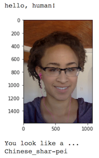
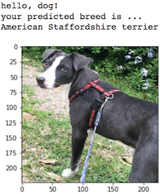
In this notebook, you will make the first steps towards developing an algorithm that could be used as part of a mobile or web app. At the end of this project, your code will accept any user-supplied image as input. If a dog is detected in the image, it will provide an estimate of the dog's breed. If a human is detected, it will provide an estimate of the dog breed that is most resembling. The image below displays potential sample output of your finished project (... but we expect that each student's algorithm will behave differently!).

Sample Dog Output

In this real-world setting, you will need to piece together a series of models to perform different tasks; for instance, the algorithm that detects humans in an image will be different from the CNN that infers dog breed. There are many points of possible failure, and no perfect algorithm exists. Your imperfect solution will nonetheless create a fun user experience!

The Road Ahead

We break the notebook into separate steps. Feel free to use the links below to navigate the notebook.

  • Step 0: Import Datasets
  • Step 1: Detect Humans
  • Step 2: Detect Dogs
  • Step 3: Create a CNN to Classify Dog Breeds (from Scratch)
  • Step 4: Create a CNN to Classify Dog Breeds (using Transfer Learning)
  • Step 5: Write your Algorithm
  • Step 6: Test Your Algorithm

Step 0: Import Datasets

Make sure that you've downloaded the required human and dog datasets:

  • Download the dog dataset. Unzip the folder and place it in this project's home directory, at the location /dogImages.

  • Download the human dataset. Unzip the folder and place it in the home directory, at location /lfw.

Note: If you are using a Windows machine, you are encouraged to use 7zip to extract the folder.

In the code cell below, we save the file paths for both the human (LFW) dataset and dog dataset in the numpy arrays human_files and dog_files.

The original notebook had the imports and set-up for plotting scattered around the notebook, but since there's so many different parts to work on it made it difficult to hunt them all down whenever I restarted the notebook so I've moved them here, but left the original imports in place (or nearly so).

Imports

In [1]:
# python
from datetime import datetime
from functools import partial
from pathlib import Path
import warnings

# from pypi
from PIL import Image, ImageFile
from tabulate import tabulate
from torchvision import datasets
import matplotlib
warnings.filterwarnings("ignore", category=matplotlib.cbook.mplDeprecation)
import cv2
import face_recognition
import matplotlib.image as matplotlib_image
import matplotlib.patches as patches
import matplotlib.pyplot as plt
import numpy as np
import seaborn
import torch
import torch.nn as nn
import torch.nn.functional as F
import torch.optim as optimizer
import torchvision.models as models
import torchvision.transforms as transforms

I tend to use the full names, but the included code uses the common practice (just not mine) of shortening numpy and pyplot so I'm going to alias them to cut down on the NameErrors.

In [2]:
pyplot = plt
numpy = np

Set Up the Plotting

In [3]:
get_ipython().run_line_magic('matplotlib', 'inline')
get_ipython().run_line_magic('config', "InlineBackend.figure_format = 'retina'")
seaborn.set(style="whitegrid",
            rc={"axes.grid": False,
                "font.family": ["sans-serif"],
                "font.sans-serif": ["Open Sans", "Latin Modern Sans", "Lato"],
                "figure.figsize": (8, 6)},
            font_scale=1)

Constants

In [4]:
INCEPTION_IMAGE_SIZE = 299
SCRATCH_IMAGE_SIZE = INCEPTION_IMAGE_SIZE
VGG_IMAGE_SIZE = 224

MEANS = [0.485, 0.456, 0.406]
DEVIATIONS = [0.229, 0.224, 0.225]
DOG_LOWER, DOG_UPPER = 150, 269

Load filenames for human and dog images.

In [5]:
ROOT_PATH = Path("~/data/datasets/dog-breed-classification/").expanduser()
HUMAN_PATH = ROOT_PATH.joinpath("lfw")
DOG_PATH = ROOT_PATH.joinpath("dogImages")
MODEL_PATH = Path("~/models/dog-breed-classification").expanduser()

assert HUMAN_PATH.is_dir()
assert DOG_PATH.is_dir()
assert MODEL_PATH.is_dir()

The MODELS is a place to store things that have been moved to the GPU so I can off-load them if needed.

In [6]:
MODELS = []

Check CUDA

In [7]:
use_cuda = torch.cuda.is_available()
device = torch.device("cuda" if use_cuda else "cpu")
print("Using {}".format(device))
Using cuda

Handle Truncated Images

In [8]:
ImageFile.LOAD_TRUNCATED_IMAGES = True
In [9]:
human_files = np.array(list(HUMAN_PATH.glob("*/*")))
dog_files = np.array(list(DOG_PATH.glob("*/*/*")))

assert len(human_files) > 0
assert len(dog_files) > 0

# print number of images in each dataset
print('There are {:,} total human images.'.format(len(human_files)))
print('There are {:,} total dog images.'.format(len(dog_files)))
There are 13,233 total human images.
There are 8,351 total dog images.

Step 1: Detect Humans

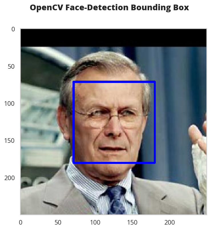
In this section, we use OpenCV's implementation of Haar feature-based cascade classifiers to detect human faces in images.

OpenCV provides many pre-trained face detectors, stored as XML files on github. We have downloaded one of these detectors and stored it in the haarcascades directory. In the next code cell, we demonstrate how to use this detector to find human faces in a sample image.

In [10]:
import cv2
import warnings
import matplotlib
warnings.filterwarnings("ignore", category=matplotlib.cbook.mplDeprecation)
import matplotlib.pyplot as plt

# extract pre-trained face detector
haar_path = ROOT_PATH.joinpath('haarcascades/haarcascade_frontalface_alt.xml')
assert haar_path.is_file()
face_cascade = cv2.CascadeClassifier(str(haar_path))

# load color (BGR) image
img = cv2.imread(str(human_files[0]))
# convert BGR image to grayscale
gray = cv2.cvtColor(img, cv2.COLOR_BGR2GRAY)

# find faces in image
faces = face_cascade.detectMultiScale(gray)

# print number of faces detected in the image
print('Number of faces detected:', len(faces))

# get bounding box for each detected face
for (x,y,w,h) in faces:
    # add bounding box to color image
    cv2.rectangle(img,(x,y),(x+w,y+h),(255,0,0),2)
    
# convert BGR image to RGB for plotting
cv_rgb = cv2.cvtColor(img, cv2.COLOR_BGR2RGB)

# display the image, along with bounding box
plt.imshow(cv_rgb)
plt.show()
Number of faces detected: 1

Before using any of the face detectors, it is standard procedure to convert the images to grayscale. The detectMultiScale function executes the classifier stored in face_cascade and takes the grayscale image as a parameter.

In the above code, faces is a numpy array of detected faces, where each row corresponds to a detected face. Each detected face is a 1D array with four entries that specifies the bounding box of the detected face. The first two entries in the array (extracted in the above code as x and y) specify the horizontal and vertical positions of the top left corner of the bounding box. The last two entries in the array (extracted here as w and h) specify the width and height of the box.

Write a Human Face Detector

We can use this procedure to write a function that returns True if a human face is detected in an image and False otherwise. This function, aptly named face_detector, takes a string-valued file path to an image as input and appears in the code block below.

In [11]:
def face_detector(img_path):
    """"returns True if face is detected in image stored at img_path"""
    img = cv2.imread(img_path)
    gray = cv2.cvtColor(img, cv2.COLOR_BGR2GRAY)
    faces = face_cascade.detectMultiScale(gray)
    return len(faces) > 0

(IMPLEMENTATION) Assess the Human Face Detector

Question 1: Use the code cell below to test the performance of the face_detector function.

  • What percentage of the first 100 images in human_files have a detected human face?
  • What percentage of the first 100 images in dog_files have a detected human face?

Ideally, we would like 100% of human images with a detected face and 0% of dog images with a detected face. You will see that our algorithm falls short of this goal, but still gives acceptable performance. We extract the file paths for the first 100 images from each of the datasets and store them in the numpy arrays human_files_short and dog_files_short.

Answer: See output below.

In [12]:
from tqdm import tqdm

human_files_short = human_files[:100]
dog_files_short = dog_files[:100]

#-#-# Do NOT modify the code above this line. #-#-#
In [13]:
set([" ".join(filename.name.split("_")[:-1]) for filename in dog_files_short])
Out[13]:
{'Afghan hound',
 'American foxhound',
 'Basset hound',
 'Belgian tervuren',
 'Bichon frise',
 'Bluetick coonhound',
 'Border terrier',
 'Boxer',
 'English cocker spaniel',
 'Greyhound',
 'Lowchen',
 'Newfoundland',
 'Norwich terrier',
 'Papillon',
 'Smooth fox terrier',
 'Tibetan mastiff'}

I'm going to re-do this again with dlib so I'll make a function to answer the question of percentages and add an f1 score to make it a little easier to compare them.

In [14]:
def species_scorer(predictor: callable,
                   true_species: list,
                   false_species: list,
                   labels: list) -> list:
    """Emit a score-table for the predictor

    Args:
     predictor: callable that returns True if it detects the expected species
     true_species: list of images that should be matched by predictor
     false_species: list of images that shouldn't be matched by predictor
     labels: column labels for the table

    Returns:
     false-positive indices
    """
    misses = [predictor(str(image)) for image in false_species]
    false_positives = sum(misses)
    true_positives = sum([predictor(str(image)) for image in true_species])
    false_negatives = len(true_species) - true_positives
    others = len(false_species)
    expected = len(true_species)
    values = ("{:.2f}%".format(100 * true_positives/expected),
            "{:.2f}%".format(100 * false_positives/others),
              "{:.2f}".format((2 * true_positives)/(2 * true_positives
                                                    + false_positives
                                                    + false_negatives)))
    table = zip(labels, values)
    print(tabulate(table, tablefmt="github", headers=["Metric", "Value"]))
    return misses
In [16]:
face_scorer = partial(species_scorer,
                      true_species=human_files_short,
                      false_species=dog_files_short,
                      labels=("First 100 images in `human_files` detected with a face",
                              "First 100 images in `dog_files` detected with a face",
                              "F1"))
In [17]:
open_cv_false_positives = face_scorer(face_detector)
Metric                                                  Value
------------------------------------------------------  -------
First 100 images in `human_files` detected with a face  98.00%
First 100 images in `dog_files` detected with a face    9.00%
F1                                                      0.95

We suggest the face detector from OpenCV as a potential way to detect human images in your algorithm, but you are free to explore other approaches, especially approaches that make use of deep learning :). Please use the code cell below to design and test your own face detection algorithm. If you decide to pursue this optional task, report performance on human_files_short and dog_files_short.

DLIB with face_recognition

This face detector uses face_recognition, a python interface to dlib's facial recognition code.

Testing It with An Image

I created the detect_faces and add_bounding_boxes functions so that I can re-use detect_faces later for the dlib version of the face_detector function.

In [18]:
def detect_faces(image_path: str) -> numpy.ndarray:
    """Finds the locations of faces
    
    Args:
     image_path: path to the image
        
    Returns:
     array of bounding box coordinates for the face(s)
    """
    image = face_recognition.load_image_file(str(image_path))
    return face_recognition.face_locations(image)
In [19]:
def add_bounding_boxes(image_path: str,
                       axe: matplotlib.axes.Axes) -> None:
    """Adds patches to the current matplotlib figure
    
    Args:
     image_path: path to the image file
     axe: axes to add the rectangle to
    """
    for (top, right, bottom, left) in detect_faces(image_path):
        width = right - left
        height = top - bottom
        rectangle = matplotlib.patches.Rectangle((top, right), width, height,
                                      fill=False)
        axe.add_patch(rectangle)
    return    
In [20]:
figure, axe = pyplot.subplots()
human = human_files[0]
name = " ".join(human.name.split("_")[:-1])
image = matplotlib.image.imread(human)
figure.suptitle("dlib Face Recognition Bounding-Box ({})".format(name),
                weight='bold')
add_bounding_boxes(human, axe)
axe.tick_params(dict(axis="both",
                     which="both",
                     bottom=False,
                     top=False))
axe.get_xaxis().set_ticks([])
axe.get_yaxis().set_ticks([])
        
plot = axe.imshow(image)

Test the performance

In [21]:
def has_face(image_path: str) -> bool:
    """Checks if there is at least one face in the image

    Args:
     image_path: path to the image file

    Returns:
     True if there's at least one face in the image
    """
    return len(detect_faces(image_path)) > 0
In [22]:
dlib_false_positives = face_scorer(has_face)
Metric                                                  Value
------------------------------------------------------  -------
First 100 images in `human_files` detected with a face  100.00%
First 100 images in `dog_files` detected with a face    11.00%
F1                                                      0.95

The DLIB version did slightly better in recognizing the humans as humans, but it also had more false positives so it did about the same overall. Although I didn't include the time the dlib version is about four times slower than the OpenCV version, so the OpenCV verision might be better in a real-time environment, on the other hand the dlib version is much simpler to use and so might be better if speed isn't a factor or recall is more important than precision.


Step 2: Detect Dogs

In this section, we use a pre-trained model to detect dogs in images.

Obtain Pre-trained VGG-16 Model

The code cell below downloads the VGG-16 model, along with weights that have been trained on ImageNet, a very large, very popular dataset used for image classification and other vision tasks. ImageNet contains over 10 million URLs, each linking to an image containing an object from one of 1000 categories.

In [22]:
import torch
import torchvision.models as models
In [22]:
# define VGG16 model
VGG16 = models.vgg16(pretrained=True)
In [23]:
# move model to GPU if CUDA is available
if use_cuda:
    VGG16 = VGG16.cuda()
    MODELS.append(VGG16)

Given an image, this pre-trained VGG-16 model returns a prediction (derived from the 1000 possible categories in ImageNet) for the object that is contained in the image.

(IMPLEMENTATION) Making Predictions with a Pre-trained Model

In the next code cell, you will write a function that accepts a path to an image (such as 'dogImages/train/001.Affenpinscher/Affenpinscher_00001.jpg') as input and returns the index corresponding to the ImageNet class that is predicted by the pre-trained VGG-16 model. The output should always be an integer between 0 and 999, inclusive.

Before writing the function, make sure that you take the time to learn how to appropriately pre-process tensors for pre-trained models in the PyTorch documentation.

Transforms

The VGG model expects a 244x244 image (Very Deep Convolutional Networks for Large-Scale Image Recognition) and according to the pytorch documentation all the pre-trained models have means [0.485, 0.456, 0.406] and standard deviations [0.229, 0.224, 0.225] so the images need to be transformed accordingly. The MEANS and DEVIATIONS lists are defined in the constants section at the top of the document along with the VGG_IMAGE_SIZE.

In [24]:
vgg_transform = transforms.Compose([transforms.Resize(255),
                                    transforms.CenterCrop(VGG_IMAGE_SIZE),
                                    transforms.ToTensor(),
                                    transforms.Normalize(MEANS,
                                                         DEVIATIONS)])

Since I'm going to use the Inception-v3 network later on I'm going to create a generic function first and then use it to build separate predictor functions.

In [25]:
def model_predict(image_path: str, model: nn.Module,
                  transform: transforms.Compose) -> int:
    """Predicts the class of item in image

    Args:
     image_path: path to the image to check
     model: model to make the prediction
     transform: callable to convert the image to a tensor

    Returns:
     index corresponding to the model's prediction
    """
    image = Image.open(str(image_path))
    image = transform(image).unsqueeze(0).to(device)
    output = model(image)
    probabilities = torch.exp(output)
    _, top_class = probabilities.topk(1, dim=1)
    return top_class.item()    
In [26]:
VGG16_predict = partial(model_predict, model=VGG16, transform=vgg_transform)

(IMPLEMENTATION) Write a Dog Detector

While looking at the dictionary, you will notice that the categories corresponding to dogs appear in an uninterrupted sequence and correspond to dictionary keys 151-268, inclusive, to include all categories from 'Chihuahua' to 'Mexican hairless'. Thus, in order to check to see if an image is predicted to contain a dog by the pre-trained VGG-16 model, we need only check if the pre-trained model predicts an index between 151 and 268 (inclusive).

Use these ideas to complete the dog_detector function below, which returns True if a dog is detected in an image (and False if not).

In [27]:
def dog_detector(img_path: str, predictor: callable=VGG16_predict) -> bool:
    """Predicts if the image is a dog

    Args:
     img_path: path to image file
     predictor: callable that maps the image to an ID
    
    Returns:
     is-dog: True if the image contains a dog
    """
    return DOG_LOWER < predictor(img_path) < DOG_UPPER

(IMPLEMENTATION) Assess the Dog Detector

Question 2: Use the code cell below to test the performance of your dog_detector function.

  • What percentage of the images in human_files_short have a detected dog?
  • What percentage of the images in dog_files_short have a detected dog?
In [28]:
dog_scorer = partial(species_scorer,
                     true_species=dog_files_short,
                     false_species=human_files_short,
                     labels=("Images in `dog_files_short` with a detected dog",
                             "Images in `human_files_short with a detected dog", "F1"))
In [30]:
false_dogs = dog_scorer(dog_detector)
Metric                                            Value
------------------------------------------------  -------
Images in `dog_files_short` with a detected dog   92.00%
Images in `human_files_short with a detected dog  1.00%
F1                                                0.95

The VGG model didn't miss any dogs but it misclassified 1% of the humans as dogs.

We suggest VGG-16 as a potential network to detect dog images in your algorithm, but you are free to explore other pre-trained networks (such as Inception-v3, ResNet-50, etc). Please use the code cell below to test other pre-trained PyTorch models. If you decide to pursue this optional task, report performance on human_files_short and dog_files_short.

Inception Dog Detector

In [29]:
inception = models.inception_v3(pretrained=True)
inception.to(device)
MODELS.append(inception)
inception.eval()
pass # this is to prevent the output from dumping into the notebook

I couldn't find anyplace where pytorch documents it, but if you look at the source code they have a comment in the forward method indicating that the image needs to be 299x299x3 so they need to be transformed to a different size from the VGG images. INCEPTION_IMAGE_SIZE is set to `299# at the top of this document since this is shared with code that comes in a later section.

In [36]:
inception_transforms = transforms.Compose([transforms.Resize(INCEPTION_IMAGE_SIZE),
                                           transforms.CenterCrop(INCEPTION_IMAGE_SIZE),
                                           transforms.ToTensor(),
                                           transforms.Normalize(MEANS,
                                                                DEVIATIONS)])
In [37]:
inception_predicts = partial(model_predict, model=inception, transform=inception_transforms)
In [38]:
inception_dog_detector = partial(dog_detector, predictor=inception_predicts)
In [39]:
dlib_false_dogs = dog_scorer(inception_dog_detector)
Metric                                            Value
------------------------------------------------  -------
Images in `dog_files_short` with a detected dog   100.00%
Images in `human_files_short with a detected dog  0.00%
F1                                                1.00

The inception model seems to do better than the VGG model did.


Step 3: Create a CNN to Classify Dog Breeds (from Scratch)

Now that we have functions for detecting humans and dogs in images, we need a way to predict breed from images. In this step, you will create a CNN that classifies dog breeds. You must create your CNN from scratch (so, you can't use transfer learning yet!), and you must attain a test accuracy of at least 10%. In Step 4 of this notebook, you will have the opportunity to use transfer learning to create a CNN that attains greatly improved accuracy.

We mention that the task of assigning breed to dogs from images is considered exceptionally challenging. To see why, consider that even a human would have trouble distinguishing between a Brittany and a Welsh Springer Spaniel.

Brittany Welsh Springer Spaniel
title

It is not difficult to find other dog breed pairs with minimal inter-class variation (for instance, Curly-Coated Retrievers and American Water Spaniels).

Curly-Coated Retriever American Water Spaniel

Likewise, recall that labradors come in yellow, chocolate, and black. Your vision-based algorithm will have to conquer this high intra-class variation to determine how to classify all of these different shades as the same breed.

Yellow Labrador Chocolate Labrador

We also mention that random chance presents an exceptionally low bar: setting aside the fact that the classes are slightly imabalanced, a random guess will provide a correct answer roughly 1 in 133 times, which corresponds to an accuracy of less than 1%.

Remember that the practice is far ahead of the theory in deep learning. Experiment with many different architectures, and trust your intuition. And, of course, have fun!

(IMPLEMENTATION) Specify Data Loaders for the Dog Dataset

Use the code cell below to write three separate data loaders for the training, validation, and test datasets of dog images (located at dogImages/train, dogImages/valid, and dogImages/test, respectively). You may find this documentation on custom datasets to be a useful resource. If you are interested in augmenting your training and/or validation data, check out the wide variety of transforms!

The SCRATCH_IMAGE_SIZE, MEANS, and DEVIATIONS variables are defined in the constants section at the top of the notebook.

In [30]:
train_transform = transforms.Compose([
    transforms.RandomRotation(30),
    transforms.RandomResizedCrop(SCRATCH_IMAGE_SIZE),
    transforms.RandomHorizontalFlip(),
    transforms.ToTensor(),
    transforms.Normalize(MEANS,
                         DEVIATIONS)])

test_transform = transforms.Compose([transforms.Resize(350),
                                     transforms.CenterCrop(SCRATCH_IMAGE_SIZE),
                                     transforms.ToTensor(),
                                     transforms.Normalize(MEANS,
                                                          DEVIATIONS)])
In [28]:
dog_training_path = DOG_PATH.joinpath("train")
dog_validation_path = DOG_PATH.joinpath("valid")
dog_testing_path = DOG_PATH.joinpath("test")
In [31]:
training = datasets.ImageFolder(root=str(dog_training_path),
                                transform=train_transform)
validation = datasets.ImageFolder(root=str(dog_validation_path),
                                  transform=test_transform)
testing = datasets.ImageFolder(root=str(dog_testing_path),
                               transform=test_transform)
In [43]:
BATCH_SIZE = 32
WORKERS = 0

train_batches = torch.utils.data.DataLoader(training, batch_size=BATCH_SIZE,
                                            shuffle=True, num_workers=WORKERS)
validation_batches = torch.utils.data.DataLoader(
    validation, batch_size=BATCH_SIZE, shuffle=True, num_workers=WORKERS)
test_batches = torch.utils.data.DataLoader(
    testing, batch_size=BATCH_SIZE, shuffle=True, num_workers=WORKERS)

loaders_scratch = dict(train=train_batches,
                       validation=validation_batches,
                       test=test_batches)

Question 3: Describe your chosen procedure for preprocessing the data.

  • How does your code resize the images (by cropping, stretching, etc)? What size did you pick for the input tensor, and why?
  • Did you decide to augment the dataset? If so, how (through translations, flips, rotations, etc)? If not, why not?

Answer:

  • The training images are resized by cropping them, while the testing images are resized by scaling then cropping them. The size I chose for the images was 299 pixels so that I can reuse them with an Inception V3 network in the next section.

  • The training was augmented using rotation, cropping, and horizontal flipping.

(IMPLEMENTATION) Model Architecture

Create a CNN to classify dog breed. Use the template in the code cell below.

In [33]:
BREEDS = len(training.classes)
print("There are {} breeds.".format(BREEDS))
There are 133 breeds.
In [14]:
LAYER_ONE_IN = 3
LAYER_ONE_OUT = 16
LAYER_TWO_OUT = LAYER_ONE_OUT * 2
LAYER_THREE_OUT = LAYER_TWO_OUT * 2
FLATTEN_TO = (SCRATCH_IMAGE_SIZE//8)**2 * LAYER_THREE_OUT
FULLY_CONNECTED_OUT = int(str(FLATTEN_TO)[:3])//100 * 100
KERNEL = 3
PADDING = 1
In [15]:
import torch.nn as nn
import torch.nn.functional as F
In [16]:
class Net(nn.Module):
    def __init__(self):
        super().__init__()
        self.conv1 = nn.Conv2d(LAYER_ONE_IN, LAYER_ONE_OUT,
                               KERNEL, padding=PADDING)
        self.conv2 = nn.Conv2d(LAYER_ONE_OUT, LAYER_TWO_OUT,
                               KERNEL, padding=PADDING)
        self.conv3 = nn.Conv2d(LAYER_TWO_OUT, LAYER_THREE_OUT,
                               KERNEL, padding=PADDING)
        # max pooling layer
        self.pool = nn.MaxPool2d(2, 2)
        # linear layer
        self.fc1 = nn.Linear(FLATTEN_TO, FULLY_CONNECTED_OUT)
        self.fc2 = nn.Linear(FULLY_CONNECTED_OUT, BREEDS)
        # dropout layer
        self.dropout = nn.Dropout(0.25)
        return
    
    def forward(self, x):
        x = self.pool(F.relu(self.conv1(x)))
        x = self.pool(F.relu(self.conv2(x)))
        x = self.pool(F.relu(self.conv3(x)))

        x = x.view(-1, FLATTEN_TO)
        x = self.dropout(x)

        x = self.dropout(F.relu(self.fc1(x)))
        return self.fc2(x)
#-#-# You so NOT have to modify the code below this line. #-#-#

# instantiate the CNN
model_scratch = Net()

# move tensors to GPU if CUDA is available
if use_cuda:
    model_scratch.cuda()
    MODELS.append(model_scratch)

Question 4: Outline the steps you took to get to your final CNN architecture and your reasoning at each step.

Answer:

It was largely trial and error, copying what we did in the CIFAR problem. I chose (somewhat arbitrarily) three convolutional layers, since two layers didn't seem to do very well. Each convolutional layer doubles the depth while halving the height and width (using MaxPool).

I then flattened the layer to transition from the convolutional layers to the fully-connected layers. I added a fully-connected layer which has 500 outputs - a rough rounding of the number of input weights of the flattened layer down to the nearest 100th. There wasn't any magic to the number, I just wanted a transition from the large flattened layer to the final output layer and when I was experimenting with larger values I was running out of memory and since this isn't the intended final model I tried to keep it modest.

To reduce the likelihood of overfitting I applied dropout to the activation layers (except the final one). Finally, at each of the layers (except the final output layer) I applied ReLU activation to make the model non-linear.

(IMPLEMENTATION) Specify Loss Function and Optimizer

Use the next code cell to specify a loss function and optimizer. Save the chosen loss function as criterion_scratch, and the optimizer as optimizer_scratch below.

In [17]:
import torch.optim as optimizer

criterion_scratch = nn.CrossEntropyLoss()
optimizer_scratch = optimizer.SGD(model_scratch.parameters(),
                                  lr=0.001,
                                  momentum=0.9)

(IMPLEMENTATION) Train and Validate the Model

Train and validate your model in the code cell below. Save the final model parameters at filepath 'model_scratch.pt'.

In [18]:
def train(n_epochs, loaders, model, optimizer, criterion, use_cuda, save_path,
          print_function: callable=print,
          is_inception: bool=False):
    """Trains the model

    Args:
     n_epochs: the number of times to repeat training
     loaders: dict of data batch-loaders
     model: the model to train
     optimizer: the gradient descent object
     criterion: The object to calculate the loss
     use_cuda: boolean to decide whether to move the data to the GPU
     save_path: path to file to save best model to
     print_function: something to pass output to
     is_inception: if True, expect a tuple of tensors as the model output
    """
    # initialize tracker for minimum validation loss
    valid_loss_min = np.Inf
    
    # check the keys are right so you don't waste an entire epoch to find out
    training_batches = loaders["train"]
    validation_batches = loaders["validation"]
    started = datetime.now()
    print_function("Training Started: {}".format(started))
    for epoch in range(1, n_epochs+1):
        # initialize variables to monitor training and validation loss
        epoch_started = datetime.now()
        train_loss = 0.0
        valid_loss = 0.0
        
        ###################
        # train the model #
        ###################
        model.train()
        for data, target in training_batches:
            # move to GPU
            if use_cuda:
                data, target = data.cuda(), target.cuda()
            optimizer.zero_grad()
            if is_inception:
                output, _ = model(data)
            else:
                output = model(data)
            loss = criterion(output, target)
            loss.backward()
            optimizer.step()
            train_loss += loss.item() * data.size(0)
        train_loss /= len(training_batches.dataset)

        ######################    
        # validate the model #
        ######################
        model.eval()
        for data, target in validation_batches:
            # move to GPU
            if use_cuda:
                data, target = data.cuda(), target.cuda()
            output = model(data)
            loss = criterion(output, target)
            valid_loss += loss.item() * data.size(0)
        valid_loss /= len(validation_batches.dataset)
        print_function('Epoch: {} \tTraining Loss: {:.6f} \tValidation Loss: {:.6f}\tElapsed: {}'.format(
            epoch,                     
            train_loss,
            valid_loss,
            datetime.now() - epoch_started,
            ))
        
        if valid_loss < valid_loss_min:
            print_function(
                ("Validation loss decreased ({:.6f} --> {:.6f}). "
                 "Saving model ...").format(
                     valid_loss_min,
                     valid_loss))
            torch.save(model.state_dict(), save_path)
            valid_loss_min = valid_loss
    ended = datetime.now()
    print_function("Training Ended: {}".format(ended))
    print_function("Total Training Time: {}".format(ended - started))            
    return model

Tee

I found out the hard way that Jupyter loses the ability to re-connect to a running cell if you close and re-open the tab, so if you do close it you will have lost all your output. This is something to make sure it gets saved to a file.

In [64]:
class Tee:
    """Save the input to a file and print it

    Args:
     log_name: name to give the log    
     directory_path: path to the directory for the file
    """
    def __init__(self, log_name: str, 
                 directory_name: str="../../../logs/dog-breed-classifier") -> None:
        self.directory_name = directory_name
        self.log_name = log_name
        self._path = None
        self._log = None
        return

    @property
    def path(self) -> Path:
        """path to the log-file"""
        if self._path is None:
            self._path = Path(self.directory_name).expanduser()
            assert self._path.is_dir()
            self._path = self._path.joinpath(self.log_name)
        return self._path

    @property
    def log(self):
        """File object to write log to"""
        if self._log is None:
            self._log = self.path.open("w", buffering=1)
        return self._log

    def __call__(self, line: str) -> None:
        """Writes to the file and stdout

        Args:
         line: text to emit
        """
        self.log.write("{}\n".format(line))
        print(line)
        return

Train the Model

In [20]:
scratch_path = MODEL_PATH.joinpath("model_scratch.pt")
scratch_log = Tee(log_name="scratch_train.log")
In [21]:
EPOCHS = 100
In [22]:
model_scratch = train(EPOCHS, loaders_scratch, model_scratch, optimizer_scratch, 
                      criterion_scratch, use_cuda, scratch_path, print_function=scratch_log)
Training Started: 2019-01-07 00:17:48.769216
Epoch: 1        Training Loss: 4.877051         Validation Loss: 4.841412       Elapsed: 0:03:13.834452
Validation loss decreased (inf --> 4.841412). Saving model ...
Epoch: 2        Training Loss: 4.820985         Validation Loss: 4.747336       Elapsed: 0:03:01.535938
Validation loss decreased (4.841412 --> 4.747336). Saving model ...
Epoch: 3        Training Loss: 4.767189         Validation Loss: 4.684055       Elapsed: 0:03:01.574621
Validation loss decreased (4.747336 --> 4.684055). Saving model ...
Epoch: 4        Training Loss: 4.728553         Validation Loss: 4.607475       Elapsed: 0:03:02.878120
Validation loss decreased (4.684055 --> 4.607475). Saving model ...
Epoch: 5        Training Loss: 4.643230         Validation Loss: 4.515298       Elapsed: 0:03:01.719175
Validation loss decreased (4.607475 --> 4.515298). Saving model ...
Epoch: 6        Training Loss: 4.601643         Validation Loss: 4.451782       Elapsed: 0:03:02.711892
Validation loss decreased (4.515298 --> 4.451782). Saving model ...
Epoch: 7        Training Loss: 4.563049         Validation Loss: 4.390049       Elapsed: 0:03:02.421659
Validation loss decreased (4.451782 --> 4.390049). Saving model ...
Epoch: 8        Training Loss: 4.525313         Validation Loss: 4.401180       Elapsed: 0:03:00.623633
Epoch: 9        Training Loss: 4.494441         Validation Loss: 4.316231       Elapsed: 0:03:03.307759
Validation loss decreased (4.390049 --> 4.316231). Saving model ...
Epoch: 10       Training Loss: 4.462459         Validation Loss: 4.309952       Elapsed: 0:03:01.247355
Validation loss decreased (4.316231 --> 4.309952). Saving model ...
Epoch: 11       Training Loss: 4.440028         Validation Loss: 4.282603       Elapsed: 0:03:01.817202
Validation loss decreased (4.309952 --> 4.282603). Saving model ...
Epoch: 12       Training Loss: 4.408276         Validation Loss: 4.256291       Elapsed: 0:03:02.940067
Validation loss decreased (4.282603 --> 4.256291). Saving model ...
Epoch: 13       Training Loss: 4.382314         Validation Loss: 4.230955       Elapsed: 0:03:01.484585
Validation loss decreased (4.256291 --> 4.230955). Saving model ...
Epoch: 14       Training Loss: 4.339535         Validation Loss: 4.178119       Elapsed: 0:03:01.819115
Validation loss decreased (4.230955 --> 4.178119). Saving model ...
Epoch: 15       Training Loss: 4.314611         Validation Loss: 4.172305       Elapsed: 0:03:01.862936
Validation loss decreased (4.178119 --> 4.172305). Saving model ...
Epoch: 16       Training Loss: 4.294925         Validation Loss: 4.179273       Elapsed: 0:03:02.859107
Epoch: 17       Training Loss: 4.269919         Validation Loss: 4.121323       Elapsed: 0:03:02.187248
Validation loss decreased (4.172305 --> 4.121323). Saving model ...
Epoch: 18       Training Loss: 4.229653         Validation Loss: 4.078084       Elapsed: 0:03:02.005417
Validation loss decreased (4.121323 --> 4.078084). Saving model ...
Epoch: 19       Training Loss: 4.211623         Validation Loss: 4.075537       Elapsed: 0:03:02.023912
Validation loss decreased (4.078084 --> 4.075537). Saving model ...
Epoch: 20       Training Loss: 4.176366         Validation Loss: 4.071403       Elapsed: 0:03:02.443931
Validation loss decreased (4.075537 --> 4.071403). Saving model ...
Epoch: 21       Training Loss: 4.162033         Validation Loss: 4.060058       Elapsed: 0:03:01.880442
Validation loss decreased (4.071403 --> 4.060058). Saving model ...
Epoch: 22       Training Loss: 4.152350         Validation Loss: 4.017785       Elapsed: 0:03:02.961102
Validation loss decreased (4.060058 --> 4.017785). Saving model ...
Epoch: 23       Training Loss: 4.126623         Validation Loss: 4.061260       Elapsed: 0:03:02.727963
Epoch: 24       Training Loss: 4.099212         Validation Loss: 3.992973       Elapsed: 0:03:01.699973
Validation loss decreased (4.017785 --> 3.992973). Saving model ...
Epoch: 25       Training Loss: 4.075190         Validation Loss: 3.998641       Elapsed: 0:03:01.713804
Epoch: 26       Training Loss: 4.046143         Validation Loss: 3.997265       Elapsed: 0:03:02.571748
Epoch: 27       Training Loss: 4.043575         Validation Loss: 3.949613       Elapsed: 0:03:01.425152
Validation loss decreased (3.992973 --> 3.949613). Saving model ...
Epoch: 28       Training Loss: 4.015487         Validation Loss: 3.961522       Elapsed: 0:03:02.782270
Epoch: 29       Training Loss: 3.998070         Validation Loss: 3.948969       Elapsed: 0:03:02.048881
Validation loss decreased (3.949613 --> 3.948969). Saving model ...
Epoch: 30       Training Loss: 3.991606         Validation Loss: 3.938675       Elapsed: 0:03:02.713836
Validation loss decreased (3.948969 --> 3.938675). Saving model ...
Epoch: 31       Training Loss: 3.963830         Validation Loss: 3.918792       Elapsed: 0:03:01.697762
Validation loss decreased (3.938675 --> 3.918792). Saving model ...
Epoch: 32       Training Loss: 3.930790         Validation Loss: 3.897582       Elapsed: 0:03:01.460303
Validation loss decreased (3.918792 --> 3.897582). Saving model ...
Epoch: 33       Training Loss: 3.896765         Validation Loss: 3.963304       Elapsed: 0:03:02.224769
Epoch: 34       Training Loss: 3.879835         Validation Loss: 3.893857       Elapsed: 0:03:02.983978
Validation loss decreased (3.897582 --> 3.893857). Saving model ...
Epoch: 35       Training Loss: 3.888119         Validation Loss: 3.900615       Elapsed: 0:03:02.187086
Epoch: 36       Training Loss: 3.839318         Validation Loss: 3.884181       Elapsed: 0:03:02.805424
Validation loss decreased (3.893857 --> 3.884181). Saving model ...
Epoch: 37       Training Loss: 3.814765         Validation Loss: 3.863985       Elapsed: 0:03:03.838610
Validation loss decreased (3.884181 --> 3.863985). Saving model ...
Epoch: 38       Training Loss: 3.801056         Validation Loss: 3.873780       Elapsed: 0:03:03.033119
Epoch: 39       Training Loss: 3.797330         Validation Loss: 3.827120       Elapsed: 0:03:02.329334
Validation loss decreased (3.863985 --> 3.827120). Saving model ...
Epoch: 40       Training Loss: 3.776431         Validation Loss: 3.852023       Elapsed: 0:03:03.616306
Epoch: 41       Training Loss: 3.747829         Validation Loss: 3.814612       Elapsed: 0:03:03.231390
Validation loss decreased (3.827120 --> 3.814612). Saving model ...
Epoch: 42       Training Loss: 3.713182         Validation Loss: 3.811580       Elapsed: 0:03:00.355972
Validation loss decreased (3.814612 --> 3.811580). Saving model ...
Epoch: 43       Training Loss: 3.705967         Validation Loss: 3.811339       Elapsed: 0:03:11.512757
Validation loss decreased (3.811580 --> 3.811339). Saving model ...
Epoch: 44       Training Loss: 3.677942         Validation Loss: 3.763790       Elapsed: 0:03:06.798942
Validation loss decreased (3.811339 --> 3.763790). Saving model ...
Epoch: 45       Training Loss: 3.670521         Validation Loss: 3.804585       Elapsed: 0:03:09.111308
Epoch: 46       Training Loss: 3.616001         Validation Loss: 3.791811       Elapsed: 0:03:07.913439
Epoch: 47       Training Loss: 3.605779         Validation Loss: 3.818132       Elapsed: 0:03:08.180969
Epoch: 48       Training Loss: 3.578845         Validation Loss: 3.802942       Elapsed: 0:03:07.502958
Epoch: 49       Training Loss: 3.569269         Validation Loss: 3.763015       Elapsed: 0:03:08.838610
Validation loss decreased (3.763790 --> 3.763015). Saving model ...
Epoch: 50       Training Loss: 3.551981         Validation Loss: 3.727734       Elapsed: 0:03:07.301504
Validation loss decreased (3.763015 --> 3.727734). Saving model ...
Epoch: 51       Training Loss: 3.539640         Validation Loss: 3.763292       Elapsed: 0:03:08.697944
Epoch: 52       Training Loss: 3.514974         Validation Loss: 3.789170       Elapsed: 0:03:07.824023
Epoch: 53       Training Loss: 3.478333         Validation Loss: 3.730328       Elapsed: 0:03:08.594196
Epoch: 54       Training Loss: 3.474018         Validation Loss: 3.710677       Elapsed: 0:03:08.306823
Validation loss decreased (3.727734 --> 3.710677). Saving model ...
Epoch: 55       Training Loss: 3.455741         Validation Loss: 3.666004       Elapsed: 0:03:07.551808
Validation loss decreased (3.710677 --> 3.666004). Saving model ...
Epoch: 56       Training Loss: 3.385648         Validation Loss: 3.755735       Elapsed: 0:03:07.685431
Epoch: 57       Training Loss: 3.391713         Validation Loss: 3.739904       Elapsed: 0:03:09.560812
Epoch: 58       Training Loss: 3.385832         Validation Loss: 3.679237       Elapsed: 0:03:07.951572
Epoch: 59       Training Loss: 3.345478         Validation Loss: 3.698172       Elapsed: 0:03:07.605253
Epoch: 61       Training Loss: 3.329898         Validation Loss: 3.687313       Elapsed: 0:03:06.961018
Epoch: 62       Training Loss: 3.332215         Validation Loss: 3.722676       Elapsed: 0:03:08.430620
Epoch: 63       Training Loss: 3.290568         Validation Loss: 3.698964       Elapsed: 0:03:08.096713
Epoch: 64       Training Loss: 3.308631         Validation Loss: 3.693485       Elapsed: 0:03:06.612021
Epoch: 65       Training Loss: 3.242924         Validation Loss: 3.676528       Elapsed: 0:03:02.644056
Epoch: 66       Training Loss: 3.210221         Validation Loss: 3.672967       Elapsed: 0:03:02.000280
Epoch: 67       Training Loss: 3.248309         Validation Loss: 3.700498       Elapsed: 0:03:02.847392
Epoch: 68       Training Loss: 3.186689         Validation Loss: 3.672294       Elapsed: 0:03:04.354137
Epoch: 69       Training Loss: 3.148231         Validation Loss: 3.709312       Elapsed: 0:03:05.193586
Epoch: 70       Training Loss: 3.167838         Validation Loss: 3.735657       Elapsed: 0:03:04.797756
Epoch: 71       Training Loss: 3.154821         Validation Loss: 3.683042       Elapsed: 0:03:07.263391
Epoch: 72       Training Loss: 3.151534         Validation Loss: 3.803930       Elapsed: 0:03:02.779610
Epoch: 73       Training Loss: 3.157296         Validation Loss: 3.690141       Elapsed: 0:03:05.410248
Epoch: 74       Training Loss: 3.101250         Validation Loss: 3.771072       Elapsed: 0:03:03.327209
Epoch: 75       Training Loss: 3.052344         Validation Loss: 3.676567       Elapsed: 0:03:01.068909
Epoch: 76       Training Loss: 3.043009         Validation Loss: 3.728986       Elapsed: 0:03:01.663287
Epoch: 77       Training Loss: 3.035244         Validation Loss: 3.787941       Elapsed: 0:03:02.757887
Epoch: 78       Training Loss: 3.024287         Validation Loss: 3.795896       Elapsed: 0:03:01.845504
Epoch: 79       Training Loss: 2.992325         Validation Loss: 3.716417       Elapsed: 0:03:02.454654
Epoch: 80       Training Loss: 2.985272         Validation Loss: 3.665017       Elapsed: 0:03:01.616717
Validation loss decreased (3.666004 --> 3.665017). Saving model ...
Epoch: 81       Training Loss: 2.972644         Validation Loss: 3.750383       Elapsed: 0:03:02.581951
Epoch: 82       Training Loss: 2.948319         Validation Loss: 3.790278       Elapsed: 0:03:02.529694
Epoch: 83       Training Loss: 2.955792         Validation Loss: 3.807737       Elapsed: 0:03:02.909021
Epoch: 84       Training Loss: 2.953483         Validation Loss: 3.884490       Elapsed: 0:03:00.926423
Epoch: 85       Training Loss: 2.907973         Validation Loss: 3.876141       Elapsed: 0:03:01.702236
Epoch: 86       Training Loss: 2.886144         Validation Loss: 3.806277       Elapsed: 0:03:02.415406
Epoch: 87       Training Loss: 2.895160         Validation Loss: 3.768452       Elapsed: 0:03:02.365341
Epoch: 88       Training Loss: 2.878172         Validation Loss: 3.794703       Elapsed: 0:03:01.910776
Epoch: 89       Training Loss: 2.850065         Validation Loss: 3.784806       Elapsed: 0:03:01.821389
Epoch: 90       Training Loss: 2.808656         Validation Loss: 3.834159       Elapsed: 0:03:02.931420
Epoch: 91       Training Loss: 2.807267         Validation Loss: 3.879032       Elapsed: 0:03:01.804976
Epoch: 92       Training Loss: 2.773044         Validation Loss: 3.779162       Elapsed: 0:03:03.069339
Epoch: 93       Training Loss: 2.787731         Validation Loss: 3.912086       Elapsed: 0:03:01.484451
Epoch: 94       Training Loss: 2.741030         Validation Loss: 3.782457       Elapsed: 0:03:01.528688
Epoch: 95       Training Loss: 2.777800         Validation Loss: 3.873816       Elapsed: 0:03:02.658232
Epoch: 96       Training Loss: 2.748137         Validation Loss: 3.923467       Elapsed: 0:03:01.510292
Epoch: 97       Training Loss: 2.725654         Validation Loss: 3.989069       Elapsed: 0:03:02.315783
Epoch: 98       Training Loss: 2.723776         Validation Loss: 3.946343       Elapsed: 0:03:01.279152
Epoch: 99       Training Loss: 2.662464         Validation Loss: 3.885177       Elapsed: 0:03:02.807385
Epoch: 100      Training Loss: 2.714636         Validation Loss: 3.916170       Elapsed: 0:03:01.294095
Training Ended: 2019-01-07 05:24:48.263423
Total Training Time: 5:06:59.494207

load the model that got the best validation accuracy

In [23]:
model_scratch.load_state_dict(torch.load(scratch_path))

(IMPLEMENTATION) Test the Model

Try out your model on the test dataset of dog images. Use the code cell below to calculate and print the test loss and accuracy. Ensure that your test accuracy is greater than 10%.

In [45]:
def test(loaders, model, criterion, use_cuda, print_function=print):

    # monitor test loss and accuracy
    test_loss = 0.
    correct = 0.
    total = 0.

    model.eval()
    for batch_idx, (data, target) in enumerate(loaders['test']):
        # move to GPU
        if use_cuda:
            data, target = data.cuda(), target.cuda()
        # forward pass: compute predicted outputs by passing inputs to the model
        output = model(data)
        # calculate the loss
        loss = criterion(output, target)
        # update average test loss 
        test_loss = test_loss + ((1 / (batch_idx + 1)) * (loss.data - test_loss))
        # convert output probabilities to predicted class
        pred = output.data.max(1, keepdim=True)[1]
        # compare predictions to true label
        correct += np.sum(np.squeeze(pred.eq(target.data.view_as(pred))).cpu().numpy())
        total += data.size(0)
            
    print_function('Test Loss: {:.6f}\n'.format(test_loss))

    print_function('\nTest Accuracy: %2d%% (%2d/%2d)' % (
        100. * correct / total, correct, total))
In [25]:
scratch_test_log = Tee("scratch_test.log")
In [ ]:
# call test function    
test(loaders_scratch, model_scratch, criterion_scratch, use_cuda, print_function=scratch_test_log)
Test Loss: 3.611238


Test Accuracy: 17% (149/836)

Step 4: Create a CNN to Classify Dog Breeds (using Transfer Learning)

You will now use transfer learning to create a CNN that can identify dog breed from images. Your CNN must attain at least 60% accuracy on the test set.

(IMPLEMENTATION) Specify Data Loaders for the Dog Dataset

Use the code cell below to write three separate data loaders for the training, validation, and test datasets of dog images (located at dogImages/train, dogImages/valid, and dogImages/test, respectively).

If you like, you are welcome to use the same data loaders from the previous step, when you created a CNN from scratch.

In [47]:
loaders_transfer = loaders_scratch

(IMPLEMENTATION) Model Architecture

Use transfer learning to create a CNN to classify dog breed. Use the code cell below, and save your initialized model as the variable model_transfer.

The Transfer Model
In [34]:
model_transfer = models.inception_v3(pretrained=True)
for parameter in model_transfer.parameters():
    parameter.requires_grad = False
classifier_inputs = model_transfer.fc.in_features
model_transfer.fc = nn.Linear(in_features=classifier_inputs,
                              out_features=BREEDS,
                              bias=True)
model_transfer.to(device)
MODELS.append(model_transfer)

Question 5: Outline the steps you took to get to your final CNN architecture and your reasoning at each step. Describe why you think the architecture is suitable for the current problem.

Answer:

I looked at the source code and the string representation of the model and saw that the classification was being done by a single fully-connected (Linear) layer with 2,048 inputs and 1,000 outputs. Since we only have 133 outputs I replaced their final layer (model.fc) with one that had the same number of inputs but only 133 outputs.

I chose the Inception V3 network because, like the VGG 16 model, it was trained on the ImageNet data-set and works to detect features in images but, as noted in Rethinking the Inception Architecture for Computer Vision, the Inception model requires fewer computational resources than the VGG model does, which I thought was an attractive feature. The Inception model does introduce a problem in that it uses an auxiliary classifier during training so the training function has to be modified to handle this (the output returns a tuple of tensors), but this seemed minor.

(IMPLEMENTATION) Specify Loss Function and Optimizer

Use the next code cell to specify a loss function and optimizer. Save the chosen loss function as criterion_transfer, and the optimizer as optimizer_transfer below.

In [ ]:
criterion_transfer = nn.CrossEntropyLoss()
optimizer_transfer = optimizer.SGD(
    model_transfer.parameters(),
    lr=0.001,
    momentum=0.9)

(IMPLEMENTATION) Train and Validate the Model

Train and validate your model in the code cell below. Save the final model parameters at filepath 'model_transfer.pt'.

In [24]:
transfer_model_path = MODEL_PATH.joinpath("model_transfer.pt")
In [65]:
transfer_log = Tee(log_name="transfer_train.log")
In [ ]:
EPOCHS = 100
In [ ]:
# train the model
model_transfer = train(EPOCHS,
                       loaders=loaders_transfer,
                       model=model_transfer,
                       optimizer=optimizer_transfer,
                       criterion=criterion_transfer,
                       use_cuda=use_cuda,
                       save_path=transfer_model_path,
                       print_function=transfer_log,
                       is_inception=True)
Training Started: 2019-01-07 05:25:10.303990
Epoch: 1        Training Loss: 4.699307         Validation Loss: 4.270935       Elapsed: 0:03:18.031065
Validation loss decreased (inf --> 4.270935). Saving model ...
Epoch: 2        Training Loss: 4.181660         Validation Loss: 3.670290       Elapsed: 0:03:17.966246
Validation loss decreased (4.270935 --> 3.670290). Saving model ...
Epoch: 3        Training Loss: 3.735970         Validation Loss: 3.142542       Elapsed: 0:03:17.943660
Validation loss decreased (3.670290 --> 3.142542). Saving model ...
Epoch: 4        Training Loss: 3.343428         Validation Loss: 2.698115       Elapsed: 0:03:18.696943
Validation loss decreased (3.142542 --> 2.698115). Saving model ...
Epoch: 5        Training Loss: 2.995878         Validation Loss: 2.334530       Elapsed: 0:03:19.205373
Validation loss decreased (2.698115 --> 2.334530). Saving model ...
Epoch: 6        Training Loss: 2.723056         Validation Loss: 2.033339       Elapsed: 0:03:19.099028
Validation loss decreased (2.334530 --> 2.033339). Saving model ...
Epoch: 7        Training Loss: 2.518057         Validation Loss: 1.812573       Elapsed: 0:03:17.994237
Validation loss decreased (2.033339 --> 1.812573). Saving model ...
Epoch: 8        Training Loss: 2.310053         Validation Loss: 1.609529       Elapsed: 0:03:16.717152
Validation loss decreased (1.812573 --> 1.609529). Saving model ...
Epoch: 9        Training Loss: 2.166829         Validation Loss: 1.439860       Elapsed: 0:03:17.935079
Validation loss decreased (1.609529 --> 1.439860). Saving model ...
Epoch: 10       Training Loss: 2.057079         Validation Loss: 1.292030       Elapsed: 0:03:17.791206
Validation loss decreased (1.439860 --> 1.292030). Saving model ...
Epoch: 11       Training Loss: 1.958263         Validation Loss: 1.243316       Elapsed: 0:03:18.748263
Validation loss decreased (1.292030 --> 1.243316). Saving model ...
Epoch: 12       Training Loss: 1.859445         Validation Loss: 1.130529       Elapsed: 0:03:17.303672
Validation loss decreased (1.243316 --> 1.130529). Saving model ...
Epoch: 13       Training Loss: 1.799369         Validation Loss: 1.067557       Elapsed: 0:03:18.150230
Validation loss decreased (1.130529 --> 1.067557). Saving model ...
Epoch: 14       Training Loss: 1.723310         Validation Loss: 1.018531       Elapsed: 0:03:18.394798
Validation loss decreased (1.067557 --> 1.018531). Saving model ...
Epoch: 15       Training Loss: 1.688872         Validation Loss: 0.965496       Elapsed: 0:03:17.432118
Validation loss decreased (1.018531 --> 0.965496). Saving model ...
Epoch: 16       Training Loss: 1.639950         Validation Loss: 0.907270       Elapsed: 0:03:17.425620
Validation loss decreased (0.965496 --> 0.907270). Saving model ...
Epoch: 17       Training Loss: 1.576800         Validation Loss: 0.875295       Elapsed: 0:03:17.972938
Validation loss decreased (0.907270 --> 0.875295). Saving model ...
Epoch: 18       Training Loss: 1.547050         Validation Loss: 0.824278       Elapsed: 0:03:18.100030
Validation loss decreased (0.875295 --> 0.824278). Saving model ...
Epoch: 19       Training Loss: 1.539646         Validation Loss: 0.808194       Elapsed: 0:03:19.895761
Validation loss decreased (0.824278 --> 0.808194). Saving model ...
Epoch: 20       Training Loss: 1.500094         Validation Loss: 0.777300       Elapsed: 0:03:18.248607
Validation loss decreased (0.808194 --> 0.777300). Saving model ...
Epoch: 21       Training Loss: 1.478536         Validation Loss: 0.762025       Elapsed: 0:03:18.096901
Validation loss decreased (0.777300 --> 0.762025). Saving model ...
Epoch: 22       Training Loss: 1.449271         Validation Loss: 0.745259       Elapsed: 0:03:17.565620
Validation loss decreased (0.762025 --> 0.745259). Saving model ...
Epoch: 23       Training Loss: 1.426696         Validation Loss: 0.721501       Elapsed: 0:03:17.674511
Validation loss decreased (0.745259 --> 0.721501). Saving model ...
Epoch: 24       Training Loss: 1.384365         Validation Loss: 0.706536       Elapsed: 0:03:18.663604
Validation loss decreased (0.721501 --> 0.706536). Saving model ...
Epoch: 25       Training Loss: 1.352370         Validation Loss: 0.684035       Elapsed: 0:03:18.739320
Validation loss decreased (0.706536 --> 0.684035). Saving model ...
Epoch: 26       Training Loss: 1.382330         Validation Loss: 0.680882       Elapsed: 0:03:18.504176
Validation loss decreased (0.684035 --> 0.680882). Saving model ...
Epoch: 27       Training Loss: 1.352410         Validation Loss: 0.662414       Elapsed: 0:03:18.004690
Validation loss decreased (0.680882 --> 0.662414). Saving model ...
Epoch: 28       Training Loss: 1.323105         Validation Loss: 0.652469       Elapsed: 0:03:17.707236
Validation loss decreased (0.662414 --> 0.652469). Saving model ...
Epoch: 29       Training Loss: 1.321770         Validation Loss: 0.634052       Elapsed: 0:03:20.164878
Validation loss decreased (0.652469 --> 0.634052). Saving model ...
Epoch: 30       Training Loss: 1.309750         Validation Loss: 0.638077       Elapsed: 0:03:21.737296
Epoch: 31       Training Loss: 1.307307         Validation Loss: 0.615018       Elapsed: 0:03:18.198152
Validation loss decreased (0.634052 --> 0.615018). Saving model ...
Epoch: 32       Training Loss: 1.259097         Validation Loss: 0.618697       Elapsed: 0:03:19.649852
Epoch: 33       Training Loss: 1.276199         Validation Loss: 0.603413       Elapsed: 0:03:16.942841
Validation loss decreased (0.615018 --> 0.603413). Saving model ...
Epoch: 34       Training Loss: 1.258176         Validation Loss: 0.589237       Elapsed: 0:03:18.103221
Validation loss decreased (0.603413 --> 0.589237). Saving model ...
Epoch: 35       Training Loss: 1.254458         Validation Loss: 0.576390       Elapsed: 0:03:18.758651
Validation loss decreased (0.589237 --> 0.576390). Saving model ...
Epoch: 36       Training Loss: 1.246464         Validation Loss: 0.571317       Elapsed: 0:03:17.794329
Validation loss decreased (0.576390 --> 0.571317). Saving model ...
Epoch: 37       Training Loss: 1.227437         Validation Loss: 0.567114       Elapsed: 0:03:17.484424
Validation loss decreased (0.571317 --> 0.567114). Saving model ...
Epoch: 38       Training Loss: 1.228403         Validation Loss: 0.557364       Elapsed: 0:03:17.744637
Validation loss decreased (0.567114 --> 0.557364). Saving model ...
Epoch: 39       Training Loss: 1.213402         Validation Loss: 0.558201       Elapsed: 0:03:17.285552
Epoch: 40       Training Loss: 1.206945         Validation Loss: 0.557859       Elapsed: 0:03:18.132396
Epoch: 41       Training Loss: 1.193073         Validation Loss: 0.536087       Elapsed: 0:03:17.725738
Validation loss decreased (0.557364 --> 0.536087). Saving model ...
Epoch: 42       Training Loss: 1.194688         Validation Loss: 0.536722       Elapsed: 0:03:17.683174
Epoch: 43       Training Loss: 1.179069         Validation Loss: 0.533558       Elapsed: 0:03:18.412587
Validation loss decreased (0.536087 --> 0.533558). Saving model ...

The connection to the server died during the training (thank you, CenturyLink) so I'll try and read the log instead.

In [28]:
with transfer_log.path.open() as reader:
    for line in reader:
        print(line.rstrip())
Training Started: 2019-01-07 05:25:10.303990
Epoch: 1        Training Loss: 4.699307         Validation Loss: 4.270935       Elapsed: 0:03:18.031065
Validation loss decreased (inf --> 4.270935). Saving model ...
Epoch: 2        Training Loss: 4.181660         Validation Loss: 3.670290       Elapsed: 0:03:17.966246
Validation loss decreased (4.270935 --> 3.670290). Saving model ...
Epoch: 3        Training Loss: 3.735970         Validation Loss: 3.142542       Elapsed: 0:03:17.943660
Validation loss decreased (3.670290 --> 3.142542). Saving model ...
Epoch: 4        Training Loss: 3.343428         Validation Loss: 2.698115       Elapsed: 0:03:18.696943
Validation loss decreased (3.142542 --> 2.698115). Saving model ...
Epoch: 5        Training Loss: 2.995878         Validation Loss: 2.334530       Elapsed: 0:03:19.205373
Validation loss decreased (2.698115 --> 2.334530). Saving model ...
Epoch: 6        Training Loss: 2.723056         Validation Loss: 2.033339       Elapsed: 0:03:19.099028
Validation loss decreased (2.334530 --> 2.033339). Saving model ...
Epoch: 7        Training Loss: 2.518057         Validation Loss: 1.812573       Elapsed: 0:03:17.994237
Validation loss decreased (2.033339 --> 1.812573). Saving model ...
Epoch: 8        Training Loss: 2.310053         Validation Loss: 1.609529       Elapsed: 0:03:16.717152
Validation loss decreased (1.812573 --> 1.609529). Saving model ...
Epoch: 9        Training Loss: 2.166829         Validation Loss: 1.439860       Elapsed: 0:03:17.935079
Validation loss decreased (1.609529 --> 1.439860). Saving model ...
Epoch: 10       Training Loss: 2.057079         Validation Loss: 1.292030       Elapsed: 0:03:17.791206
Validation loss decreased (1.439860 --> 1.292030). Saving model ...
Epoch: 11       Training Loss: 1.958263         Validation Loss: 1.243316       Elapsed: 0:03:18.748263
Validation loss decreased (1.292030 --> 1.243316). Saving model ...
Epoch: 12       Training Loss: 1.859445         Validation Loss: 1.130529       Elapsed: 0:03:17.303672
Validation loss decreased (1.243316 --> 1.130529). Saving model ...
Epoch: 13       Training Loss: 1.799369         Validation Loss: 1.067557       Elapsed: 0:03:18.150230
Validation loss decreased (1.130529 --> 1.067557). Saving model ...
Epoch: 14       Training Loss: 1.723310         Validation Loss: 1.018531       Elapsed: 0:03:18.394798
Validation loss decreased (1.067557 --> 1.018531). Saving model ...
Epoch: 15       Training Loss: 1.688872         Validation Loss: 0.965496       Elapsed: 0:03:17.432118
Validation loss decreased (1.018531 --> 0.965496). Saving model ...
Epoch: 16       Training Loss: 1.639950         Validation Loss: 0.907270       Elapsed: 0:03:17.425620
Validation loss decreased (0.965496 --> 0.907270). Saving model ...
Epoch: 17       Training Loss: 1.576800         Validation Loss: 0.875295       Elapsed: 0:03:17.972938
Validation loss decreased (0.907270 --> 0.875295). Saving model ...
Epoch: 18       Training Loss: 1.547050         Validation Loss: 0.824278       Elapsed: 0:03:18.100030
Validation loss decreased (0.875295 --> 0.824278). Saving model ...
Epoch: 19       Training Loss: 1.539646         Validation Loss: 0.808194       Elapsed: 0:03:19.895761
Validation loss decreased (0.824278 --> 0.808194). Saving model ...
Epoch: 20       Training Loss: 1.500094         Validation Loss: 0.777300       Elapsed: 0:03:18.248607
Validation loss decreased (0.808194 --> 0.777300). Saving model ...
Epoch: 21       Training Loss: 1.478536         Validation Loss: 0.762025       Elapsed: 0:03:18.096901
Validation loss decreased (0.777300 --> 0.762025). Saving model ...
Epoch: 22       Training Loss: 1.449271         Validation Loss: 0.745259       Elapsed: 0:03:17.565620
Validation loss decreased (0.762025 --> 0.745259). Saving model ...
Epoch: 23       Training Loss: 1.426696         Validation Loss: 0.721501       Elapsed: 0:03:17.674511
Validation loss decreased (0.745259 --> 0.721501). Saving model ...
Epoch: 24       Training Loss: 1.384365         Validation Loss: 0.706536       Elapsed: 0:03:18.663604
Validation loss decreased (0.721501 --> 0.706536). Saving model ...
Epoch: 25       Training Loss: 1.352370         Validation Loss: 0.684035       Elapsed: 0:03:18.739320
Validation loss decreased (0.706536 --> 0.684035). Saving model ...
Epoch: 26       Training Loss: 1.382330         Validation Loss: 0.680882       Elapsed: 0:03:18.504176
Validation loss decreased (0.684035 --> 0.680882). Saving model ...
Epoch: 27       Training Loss: 1.352410         Validation Loss: 0.662414       Elapsed: 0:03:18.004690
Validation loss decreased (0.680882 --> 0.662414). Saving model ...
Epoch: 28       Training Loss: 1.323105         Validation Loss: 0.652469       Elapsed: 0:03:17.707236
Validation loss decreased (0.662414 --> 0.652469). Saving model ...
Epoch: 29       Training Loss: 1.321770         Validation Loss: 0.634052       Elapsed: 0:03:20.164878
Validation loss decreased (0.652469 --> 0.634052). Saving model ...
Epoch: 30       Training Loss: 1.309750         Validation Loss: 0.638077       Elapsed: 0:03:21.737296
Epoch: 31       Training Loss: 1.307307         Validation Loss: 0.615018       Elapsed: 0:03:18.198152
Validation loss decreased (0.634052 --> 0.615018). Saving model ...
Epoch: 32       Training Loss: 1.259097         Validation Loss: 0.618697       Elapsed: 0:03:19.649852
Epoch: 33       Training Loss: 1.276199         Validation Loss: 0.603413       Elapsed: 0:03:16.942841
Validation loss decreased (0.615018 --> 0.603413). Saving model ...
Epoch: 34       Training Loss: 1.258176         Validation Loss: 0.589237       Elapsed: 0:03:18.103221
Validation loss decreased (0.603413 --> 0.589237). Saving model ...
Epoch: 35       Training Loss: 1.254458         Validation Loss: 0.576390       Elapsed: 0:03:18.758651
Validation loss decreased (0.589237 --> 0.576390). Saving model ...
Epoch: 36       Training Loss: 1.246464         Validation Loss: 0.571317       Elapsed: 0:03:17.794329
Validation loss decreased (0.576390 --> 0.571317). Saving model ...
Epoch: 37       Training Loss: 1.227437         Validation Loss: 0.567114       Elapsed: 0:03:17.484424
Validation loss decreased (0.571317 --> 0.567114). Saving model ...
Epoch: 38       Training Loss: 1.228403         Validation Loss: 0.557364       Elapsed: 0:03:17.744637
Validation loss decreased (0.567114 --> 0.557364). Saving model ...
Epoch: 39       Training Loss: 1.213402         Validation Loss: 0.558201       Elapsed: 0:03:17.285552
Epoch: 40       Training Loss: 1.206945         Validation Loss: 0.557859       Elapsed: 0:03:18.132396
Epoch: 41       Training Loss: 1.193073         Validation Loss: 0.536087       Elapsed: 0:03:17.725738
Validation loss decreased (0.557364 --> 0.536087). Saving model ...
Epoch: 42       Training Loss: 1.194688         Validation Loss: 0.536722       Elapsed: 0:03:17.683174
Epoch: 43       Training Loss: 1.179069         Validation Loss: 0.533558       Elapsed: 0:03:18.412587
Validation loss decreased (0.536087 --> 0.533558). Saving model ...
Epoch: 44       Training Loss: 1.173093         Validation Loss: 0.521101       Elapsed: 0:03:17.631464
Validation loss decreased (0.533558 --> 0.521101). Saving model ...
Epoch: 45       Training Loss: 1.153653         Validation Loss: 0.527879       Elapsed: 0:03:17.595422
Epoch: 46       Training Loss: 1.158538         Validation Loss: 0.535613       Elapsed: 0:03:18.427818
Epoch: 47       Training Loss: 1.174377         Validation Loss: 0.528422       Elapsed: 0:03:17.892116
Epoch: 48       Training Loss: 1.164288         Validation Loss: 0.507026       Elapsed: 0:03:17.780444
Validation loss decreased (0.521101 --> 0.507026). Saving model ...
Epoch: 49       Training Loss: 1.161782         Validation Loss: 0.503888       Elapsed: 0:03:17.422116
Validation loss decreased (0.507026 --> 0.503888). Saving model ...
Epoch: 50       Training Loss: 1.163059         Validation Loss: 0.500597       Elapsed: 0:03:17.825155
Validation loss decreased (0.503888 --> 0.500597). Saving model ...
Epoch: 51       Training Loss: 1.154003         Validation Loss: 0.509676       Elapsed: 0:03:17.683708
Epoch: 52       Training Loss: 1.122364         Validation Loss: 0.500437       Elapsed: 0:03:16.342809
Validation loss decreased (0.500597 --> 0.500437). Saving model ...
Epoch: 53       Training Loss: 1.118776         Validation Loss: 0.502778       Elapsed: 0:03:17.775326
Epoch: 54       Training Loss: 1.137227         Validation Loss: 0.489028       Elapsed: 0:03:16.730713
Validation loss decreased (0.500437 --> 0.489028). Saving model ...
Epoch: 55       Training Loss: 1.112989         Validation Loss: 0.490746       Elapsed: 0:03:17.194025
Epoch: 56       Training Loss: 1.112278         Validation Loss: 0.491313       Elapsed: 0:03:18.037435
Epoch: 57       Training Loss: 1.105172         Validation Loss: 0.488087       Elapsed: 0:03:17.750197
Validation loss decreased (0.489028 --> 0.488087). Saving model ...
Epoch: 58       Training Loss: 1.106263         Validation Loss: 0.477318       Elapsed: 0:03:17.918800
Validation loss decreased (0.488087 --> 0.477318). Saving model ...
Epoch: 59       Training Loss: 1.110798         Validation Loss: 0.484890       Elapsed: 0:03:17.959631
Epoch: 60       Training Loss: 1.102846         Validation Loss: 0.475269       Elapsed: 0:03:17.318802
Validation loss decreased (0.477318 --> 0.475269). Saving model ...
Epoch: 61       Training Loss: 1.107576         Validation Loss: 0.470764       Elapsed: 0:03:17.191263
Validation loss decreased (0.475269 --> 0.470764). Saving model ...
Epoch: 62       Training Loss: 1.079003         Validation Loss: 0.469544       Elapsed: 0:03:17.907726
Validation loss decreased (0.470764 --> 0.469544). Saving model ...
Epoch: 63       Training Loss: 1.085582         Validation Loss: 0.473371       Elapsed: 0:03:17.590775
Epoch: 64       Training Loss: 1.097795         Validation Loss: 0.466651       Elapsed: 0:03:16.782743
Validation loss decreased (0.469544 --> 0.466651). Saving model ...
Epoch: 65       Training Loss: 1.087516         Validation Loss: 0.466158       Elapsed: 0:03:18.581609
Validation loss decreased (0.466651 --> 0.466158). Saving model ...
Epoch: 66       Training Loss: 1.041934         Validation Loss: 0.469748       Elapsed: 0:03:17.901108
Epoch: 67       Training Loss: 1.075575         Validation Loss: 0.454066       Elapsed: 0:03:17.029518
Validation loss decreased (0.466158 --> 0.454066). Saving model ...
Epoch: 68       Training Loss: 1.074739         Validation Loss: 0.474331       Elapsed: 0:03:18.015337
Epoch: 69       Training Loss: 1.052330         Validation Loss: 0.461796       Elapsed: 0:03:17.474546
Epoch: 70       Training Loss: 1.074078         Validation Loss: 0.457424       Elapsed: 0:03:16.963451
Epoch: 71       Training Loss: 1.032617         Validation Loss: 0.449744       Elapsed: 0:03:17.340017
Validation loss decreased (0.454066 --> 0.449744). Saving model ...
Epoch: 72       Training Loss: 1.054414         Validation Loss: 0.454565       Elapsed: 0:03:17.676010
Epoch: 73       Training Loss: 1.044849         Validation Loss: 0.453206       Elapsed: 0:03:17.600106
Epoch: 74       Training Loss: 1.035498         Validation Loss: 0.458112       Elapsed: 0:03:17.464877
Epoch: 75       Training Loss: 1.047880         Validation Loss: 0.459989       Elapsed: 0:03:17.049121
Epoch: 76       Training Loss: 1.034578         Validation Loss: 0.446105       Elapsed: 0:03:18.764851
Validation loss decreased (0.449744 --> 0.446105). Saving model ...
Epoch: 77       Training Loss: 1.032169         Validation Loss: 0.439367       Elapsed: 0:03:18.741754
Validation loss decreased (0.446105 --> 0.439367). Saving model ...
Epoch: 78       Training Loss: 1.048666         Validation Loss: 0.448395       Elapsed: 0:03:17.824941
Epoch: 79       Training Loss: 1.040212         Validation Loss: 0.440193       Elapsed: 0:03:18.251639
Epoch: 80       Training Loss: 1.032011         Validation Loss: 0.441098       Elapsed: 0:03:17.759952
Epoch: 81       Training Loss: 1.038431         Validation Loss: 0.434215       Elapsed: 0:03:16.541620
Validation loss decreased (0.439367 --> 0.434215). Saving model ...
Epoch: 82       Training Loss: 1.039337         Validation Loss: 0.442144       Elapsed: 0:03:17.911105
Epoch: 83       Training Loss: 1.032783         Validation Loss: 0.438590       Elapsed: 0:03:17.591553
Epoch: 84       Training Loss: 1.034323         Validation Loss: 0.441891       Elapsed: 0:03:17.387050
Epoch: 85       Training Loss: 1.055545         Validation Loss: 0.434267       Elapsed: 0:03:17.262275
Epoch: 86       Training Loss: 0.996985         Validation Loss: 0.432956       Elapsed: 0:03:17.287156
Validation loss decreased (0.434215 --> 0.432956). Saving model ...
Epoch: 87       Training Loss: 1.025106         Validation Loss: 0.433783       Elapsed: 0:03:17.746683
Epoch: 88       Training Loss: 1.003464         Validation Loss: 0.436888       Elapsed: 0:03:17.344770
Epoch: 89       Training Loss: 1.021132         Validation Loss: 0.432445       Elapsed: 0:03:18.347353
Validation loss decreased (0.432956 --> 0.432445). Saving model ...
Epoch: 90       Training Loss: 1.025346         Validation Loss: 0.428862       Elapsed: 0:03:18.518516
Validation loss decreased (0.432445 --> 0.428862). Saving model ...
Epoch: 91       Training Loss: 1.039084         Validation Loss: 0.418361       Elapsed: 0:03:18.556944
Validation loss decreased (0.428862 --> 0.418361). Saving model ...
Epoch: 92       Training Loss: 1.009550         Validation Loss: 0.424567       Elapsed: 0:03:17.763665
Epoch: 93       Training Loss: 1.002043         Validation Loss: 0.430174       Elapsed: 0:03:17.460125
Epoch: 94       Training Loss: 0.995485         Validation Loss: 0.417896       Elapsed: 0:03:18.836221
Validation loss decreased (0.418361 --> 0.417896). Saving model ...
Epoch: 95       Training Loss: 0.969755         Validation Loss: 0.419555       Elapsed: 0:03:11.488185
Epoch: 96       Training Loss: 0.987362         Validation Loss: 0.421185       Elapsed: 0:03:10.406026
Epoch: 97       Training Loss: 0.980267         Validation Loss: 0.417785       Elapsed: 0:03:10.542342
Validation loss decreased (0.417896 --> 0.417785). Saving model ...
Epoch: 98       Training Loss: 0.973978         Validation Loss: 0.416819       Elapsed: 0:03:12.167687
Validation loss decreased (0.417785 --> 0.416819). Saving model ...
Epoch: 99       Training Loss: 0.994163         Validation Loss: 0.418498       Elapsed: 0:03:17.225706
Epoch: 100      Training Loss: 0.998819         Validation Loss: 0.423518       Elapsed: 0:03:18.415953
Training Ended: 2019-01-07 10:55:04.465024
Total Training Time: 5:29:54.161034
In [25]:
# load the model that got the best validation accuracy (uncomment the line below)
model_transfer.load_state_dict(torch.load(transfer_model_path))
---------------------------------------------------------------------------
RuntimeError                              Traceback (most recent call last)
<ipython-input-25-bac3efba0fcd> in <module>
      1 # load the model that got the best validation accuracy (uncomment the line below)
----> 2 model_transfer.load_state_dict(torch.load(transfer_model_path))

~/.virtualenvs/neural_networks/lib/python3.6/site-packages/torch/nn/modules/module.py in load_state_dict(self, state_dict, strict)
    717         if len(error_msgs) > 0:
    718             raise RuntimeError('Error(s) in loading state_dict for {}:\n\t{}'.format(
--> 719                                self.__class__.__name__, "\n\t".join(error_msgs)))
    720 
    721     def parameters(self):

RuntimeError: Error(s) in loading state_dict for Inception3:
        size mismatch for fc.weight: copying a param of torch.Size([1000, 2048]) from checkpoint, where the shape is torch.Size([133, 2048]) in current model.
        size mismatch for fc.bias: copying a param of torch.Size([1000]) from checkpoint, where the shape is torch.Size([133]) in current model.

(IMPLEMENTATION) Test the Model

Try out your model on the test dataset of dog images. Use the code cell below to calculate and print the test loss and accuracy. Ensure that your test accuracy is greater than 60%.

In [46]:
transfer_test_log = Tee("transfer_test.log")
In [51]:
test(loaders_transfer, model_transfer, criterion_transfer, use_cuda, print_function=transfer_test_log)
Test Loss: 0.425383


Test Accuracy: 87% (734/836)

(IMPLEMENTATION) Predict Dog Breed with the Model

Write a function that takes an image path as input and returns the dog breed (Affenpinscher, Afghan hound, etc) that is predicted by your model.

In [32]:
class_names = [item[4:].replace("_", " ") for item in training.classes]

def predict_breed_transfer(img_path: str) -> str:
    """Predicts the dog-breed of what's in the image

    Args:
     img_path: path to the image to search

    Returns:
     the name of the dog-breed
    """
    # load the image
    image = Image.open(image_path)

    # convert the image to a tensor
    tensor = test_transform(image)

    # add a batch number
    tensor = tensor.unsqueeze_(0)

    # put on the GPU or CPU
    tensor = tensor.to(device)

    # make it a variable
    x = torch.autograd.Variable(tensor)

    # make the prediction
    output = model(x)
    return class_names[output.data.cpu().numpy().argmax()]

Step 5: Write your Algorithm

Write an algorithm that accepts a file path to an image and first determines whether the image contains a human, dog, or neither. Then,

  • if a dog is detected in the image, return the predicted breed.
  • if a human is detected in the image, return the resembling dog breed.
  • if neither is detected in the image, provide output that indicates an error.

You are welcome to write your own functions for detecting humans and dogs in images, but feel free to use the face_detector and human_detector functions developed above. You are required to use your CNN from Step 4 to predict dog breed.

Some sample output for our algorithm is provided below, but feel free to design your own user experience!

Sample Human Output

(IMPLEMENTATION) Write your Algorithm

Re-Done Code

I originally wrote my implementation using classes, because I kept getting errors related to the fact that jupyter lets you run cells out of order so I wanted them defined as a group (and because I find it easier to work this way once there is this much code). So I broke the parts up to answer the questions but am including them in this section to make my final solution work. Everything until the Dog Breed Classifier section was already implemented in the sections above using functions and global variables instead of class methods, only the Dog Breed Classification section and below has new implementations.

In [53]:
class Transformer:
    """Builds the image transformers

    Args:
     means: list of means for each channel
     deviations: list of standard deviations for each channel
     image_size: size to crop the image to
    """
    def __init__(self,
                 means: list=MEANS,
                 deviations: list=DEVIATIONS,
                 image_size: int=INCEPTION_IMAGE_SIZE) -> None:
        self.means = means
        self.deviations = deviations
        self.image_size = image_size
        self._training = None
        self._testing = None
        return

    @property
    def training(self) -> transforms.Compose:
        """The image transformers for the training"""
        if self._training is None:
            self._training = transforms.Compose([
                transforms.RandomRotation(30),
                transforms.RandomResizedCrop(self.image_size),
                transforms.RandomHorizontalFlip(),
                transforms.ToTensor(),
                transforms.Normalize(self.means,
                                     self.deviations)])
        return self._training

    @property
    def testing(self) -> transforms.Compose:
        """Image transforms for the testing"""
        if self._testing is None:
            self._testing = transforms.Compose(
                [transforms.Resize(self.image_size),
                 transforms.CenterCrop(INCEPTION_IMAGE_SIZE),
                 transforms.ToTensor(),
                 transforms.Normalize(self.means,
                                      self.deviations)])
        return self._testing
In [54]:
class DogDetector:
    """Detects dogs

    Args:
     model_definition: definition for the model
     device: where to run the model (CPU or CUDA)
     image_size: what to resize the file to (depends on the model-definition)
     means: mean for each channel
     deviations: standard deviation for each channel
     dog_lower_bound: index below where dogs start
     dog_upper_bound: index above where dogs end
    """
    def __init__(self,
                 model_definition: nn.Module=models.inception_v3,
                 image_size: int=INCEPTION_IMAGE_SIZE,
                 means: list=MEANS,
                 deviations: list=DEVIATIONS,
                 dog_lower_bound: int=DOG_LOWER,
                 dog_upper_bound: int=DOG_UPPER,
                 device: torch.device=None) -> None:
        self.model_definition = model_definition
        self.image_size = image_size
        self.means = means
        self.deviations = deviations
        self.dog_lower_bound = dog_lower_bound
        self.dog_upper_bound = dog_upper_bound
        self._device = device
        self._model = None
        self._transformer = None
        return

    @property
    def device(self) -> torch.device:
        """The device to add the model to"""
        if self._device is None:
            self._device = torch.device("cuda"
                                        if torch.cuda.is_available()
                                        else "cpu")
        return self._device

    @property
    def model(self) -> nn.Module:
        """Build the model"""
        if self._model is None:
            self._model = self.model_definition(pretrained=True)
            self._model.to(self.device)
            self._model.eval()
        return self._model

    @property
    def transformer(self) -> Transformer:
        """The transformer for the image data"""
        if self._transformer is None:
            self._transformer = Transformer()
        return self._transformer

    def __call__(self, image_path: str) -> bool:
        """Checks if there is a dog in the image"""
        image = Image.open(str(image_path))
        image = self.transformer.testing(image).unsqueeze(0).to(self.device)
        output = self.model(image)
        probabilities = torch.exp(output)
        _, top_class = probabilities.topk(1, dim=1)
        return self.dog_lower_bound < top_class.item() < self.dog_upper_bound
In [55]:
class SpeciesDetector:
    """Detect dogs and humans

    Args:
     device: where to put the dog-detecting model
    """
    def __init__(self, device: torch.device=None) -> None:
        self.device = device
        self._dog_detector = None
        return

    @property
    def dog_detector(self) -> DogDetector:
        """Neural Network dog-detector"""
        if self._dog_detector is None:
            self._dog_detector = DogDetector(device=self.device)
        return self._dog_detector

    def is_human(self, image_path: str) -> bool:
        """Checks if the image is a human
        
        Args:
         image_path: path to the image

        Returns:
         True if there is a human face in the image
        """
        image = face_recognition.load_image_file(str(image_path))
        faces = face_recognition.face_locations(image)
        return len(faces) > 0

    def is_dog(self, image_path: str) -> bool:        
        """Checks if there is a dog in the image"""
        return self.dog_detector(image_path)
In [56]:
class DogPaths:
    """holds the paths to the dog images"""
    def __init__(self) -> None:
        self._main = None
        self._training = None
        self._testing = None
        self._validation = None
        return

    @property
    def main(self) -> Path:
        """The path to the main folder"""
        if self._main is None:
            self._main = DOG_PATH
        return self._main

    @property
    def training(self) -> Path:
        """Path to the training images"""
        if self._training is None:
            self._training = DOG_PATH.joinpath("train")
        return self._training

    @property
    def validation(self) -> Path:
        """Path to the validation images"""
        if self._validation is None:
            self._validation = DOG_PATH.joinpath("valid")
        return self._validation

    @property
    def testing(self) -> Path:
        """Path to the testing images"""
        if self._testing is None:
            self._testing = DOG_PATH.joinpath("test")
        return self._testing
In [57]:
class Inception:
    """Sets up the model, criterion, and optimizer for the transfer learning

    Args:
     classes: number of outputs for the final layer
     device: processor to use
     model_path: path to a saved model
     learning_rate: learning rate for the optimizer
     momentum: momentum for the optimizer
    """
    def __init__(self, classes: int,
                 device: torch.device=None,
                 model_path: str=None,
                 learning_rate: float=0.001, momentum: float=0.9) -> None:
        self.classes = classes
        self.model_path = model_path
        self.learning_rate = learning_rate
        self.momentum = momentum
        self._device = device
        self._model = None
        self._classifier_inputs = None
        self._criterion = None
        self._optimizer = None
        return

    @property
    def device(self) -> torch.device:
        """Processor to use (cpu or cuda)"""
        if self._device is None:
            self._device = torch.device(
                "cuda" if torch.cuda.is_available() else "cpu")
        return self._device

    @property
    def model(self) -> models.inception_v3:
        """The inception model"""
        if self._model is None:
            self._model = models.inception_v3(pretrained=True)
            for parameter in self._model.parameters():
                parameter.requires_grad = False
            classifier_inputs = self._model.fc.in_features
            self._model.fc = nn.Linear(in_features=classifier_inputs,
                                       out_features=self.classes,
                                       bias=True)
            self._model.to(self.device)
            if self.model_path:
                self._model.load_state_dict(torch.load(self.model_path))
        return self._model

    @property
    def criterion(self) -> nn.CrossEntropyLoss:
        """The loss callable"""
        if self._criterion is None:
            self._criterion = nn.CrossEntropyLoss()
        return self._criterion

    @property
    def optimizer(self) -> optimizer.SGD:
        """The Gradient Descent object"""
        if self._optimizer is None:
            self._optimizer = optimizer.SGD(
                self.model.parameters(),
                lr=self.learning_rate,
                momentum=self.momentum)
        return self._optimizer
In [58]:
class DataSets:
    """Builds the data-sets

    Args:
     paths: object with the paths to the data-sets
    """
    def __init__(self, paths: DogPaths=None, transformer: Transformer=None) -> None:
        self._paths = paths
        self._transformer = transformer
        self._training = None
        self._validation = None
        self._testing = None
        return

    @property
    def paths(self) -> DogPaths:
        """Object with the paths to the image files"""
        if self._paths is None:
            self._paths = DogPaths()
        return self._paths

    @property
    def transformer(self) -> Transformer:
        """Object with the image transforms"""
        if self._transformer is None:
            self._transformer = Transformer()
        return self._transformer

    @property
    def training(self) -> datasets.ImageFolder:
        """The training data set"""
        if self._training is None:
            self._training = datasets.ImageFolder(
                root=self.paths.training,
                transform=self.transformer.training)
        return self._training

    @property
    def validation(self) -> datasets.ImageFolder:
        """The validation dataset"""
        if self._validation is None:
            self._validation = datasets.ImageFolder(
                root=self.paths.validation,
                transform=self.transformer.testing)
        return self._validation

    @property
    def testing(self) -> datasets.ImageFolder:
        """The test set"""
        if self._testing is None:
            self._testing = datasets.ImageFolder(
                root=self.paths.testing,
                transform=self.transformer.testing)
        return self._testing
In [59]:
class DogPredictor:
    """Makes dog-breed predictions
    
    Args:
     model_path: path to the model's state-dict
     device: processor to run the model on
     data_sets: a DataSets object
     inception: an Inception object
    """
    def __init__(self, model_path: str=None,
                 device: torch.device=None,
                 data_sets: DataSets=None,
                 inception: Inception=None) -> None:
        self.model_path = model_path
        self.device = device
        self._data_sets = data_sets
        self._inception = inception
        self._breeds = None
        return

    @property
    def data_sets(self) -> DataSets:
        if self._data_sets is None:
            self._data_sets = DataSets()
        return self._data_sets

    @property
    def inception(self) -> Inception:
        """An Inception object"""
        if self._inception is None:
            self._inception = Inception(
                classes=len(self.data_sets.training.classes),
                model_path=self.model_path,
                device=self.device)
            self._inception.model.eval()
        return self._inception

    @property
    def breeds(self) -> list:
        """A list of dog-breeds"""
        if self._breeds is None:
            self._breeds = [name[4:].replace("_", " ")
                            for name in self.data_sets.training.classes]
        return self._breeds

    def predict_index(self, image_path:str) -> int:
        """Predicts the index of the breed of the dog in the image

        Args:
         image_path: path to the image
        Returns:
         index in the breeds list for the image
        """
        model = self.inception.model        
        image = Image.open(image_path)
        tensor = self.data_sets.transformer.testing(image)
        # add a batch number
        tensor = tensor.unsqueeze_(0)
        tensor = tensor.to(self.inception.device)
        x = torch.autograd.Variable(tensor)
        output = model(x)
        return output.data.cpu().numpy().argmax()

    def __call__(self, image_path) -> str:
        """Predicts the breed of the dog in the image

        Args:
         image_path: path to the image
        Returns:
         name of the breed
        """
        return self.breeds[self.predict_index(image_path)]

The Dog Breed Classifier

This implements the dog-breed classifier using the classes immediately above.

In [60]:
class DogBreedClassifier:
    """Tries To predict the dog-breed for an image

    Args:
     model_path: path to the inception-model
    """
    def __init__(self, model_path: str) -> None:
        self.model_path = model_path
        self._breed_predictor = None
        self._species_detector = None
        return

    @property
    def breed_predictor(self) -> DogPredictor:
        """Predictor of dog-breeds"""
        if self._breed_predictor is None:
            self._breed_predictor = DogPredictor(model_path=self.model_path)
        return self._breed_predictor

    @property
    def species_detector(self) -> SpeciesDetector:
        """Detector of humans and dogs"""
        if self._species_detector is None:
            self._species_detector = SpeciesDetector(
                device=self.breed_predictor.inception.device)
        return self._species_detector

    def render(self, image_path: str, species: str, breed: str) -> None:
        """Renders the image

        Args:
         image_path: path to the image to render
         species: identified species
         breed: identified breed
        """
        name = " ".join(image_path.name.split(".")[0].split("_")).title()
        figure, axe = pyplot.subplots()
        figure.suptitle("{} ({})".format(species, name), weight="bold")
        axe.set_xlabel("Looks like a {}.".format(breed))
        image = Image.open(image_path)
        axe.tick_params(dict(axis="both",
                             which="both",
                             bottom=False,
                             top=False))
        axe.get_xaxis().set_ticks([])
        axe.get_yaxis().set_ticks([])
        axe_image = axe.imshow(image)
        return

    def __call__(self, image_path:str) -> None:
        """detects the dog-breed and displays the image

        Args:
         image_path: path to the image
        """
        image_path = Path(image_path)
        is_dog = self.species_detector.is_dog(image_path)
        is_human = self.species_detector.is_human(image_path)

        if not is_dog and not is_human:
            species = "Error: Neither Human nor Dog"
            breed = "?"
        else:
            breed = self.breed_predictor(image_path)

        if is_dog and is_human:
            species = "Human-Dog Hybrid"
        elif is_dog:
            species = "Dog"
        elif is_human:
            species = "Human"
        self.render(image_path, species, breed)
        return

The next cell transfers the existing models to the CPU to free up memory on the GPU, since the class-based version builds them anyway.

In [67]:
for model in MODELS:
    model.cpu()
classifier = DogBreedClassifier(model_path=transfer_model_path)
In [68]:
def run_app(img_path):
    """Runs the dog breed classifier

    Args:
     img_path: path to the image to classify
    """
    classifier(img_path)
    return

Step 6: Test Your Algorithm

In this section, you will take your new algorithm for a spin! What kind of dog does the algorithm think that you look like? If you have a dog, does it predict your dog's breed accurately? If you have a cat, does it mistakenly think that your cat is a dog?

(IMPLEMENTATION) Test Your Algorithm on Sample Images!

Test your algorithm at least six images on your computer. Feel free to use any images you like. Use at least two human and two dog images.

First, I'll create a function to find species detections that were wrong.

In [12]:
def first_prediction(source: list, start:int=0, count: int=1) -> int:
    """Gets the index of the first True prediction

    Args:
     source: list of True/False predictions
     start: index to start the search from
     count: number of indices to find

    Returns:
     indices of first True predictions found
    """
    indices = []
    found = 0
    for index, prediction in enumerate(source[start:]):
        if prediction:
            print("{}: {}".format(start + index, prediction))
            indices.append(index)
            found += 1
            if found == count:
                break
    return indices
In [37]:
human_dog = first_prediction(dlib_false_positives)
0: True
In [38]:
hot_dog = "hot_dog.jpg"
rabbit = "rabbit.jpg"
test_images = [dog_files_short[human_dog[0]], hot_dog, rabbit]
In [39]:
dogs = numpy.random.choice(dog_files, 3)
humans = numpy.random.choice(human_files, 3)
In [71]:
images = numpy.hstack((dogs, humans, test_images))
for image in images:
    run_app(image)

Question 6: Is the output better than you expected :) ? Or worse :( ? Provide at least three possible points of improvement for your algorithm.

Answer: (Three possible points for improvement) The outcome was better than I expected, but here are some possible improvements:

  1. Try other models, in particular the Resnet model which is the state-of-the art for imagenet.
  2. Tune the Transfer Model more - it improved at epoch 98 so it might do better with more training (I stopped because of the time it took to train it).
  3. Try alternatives to Stochastic Gradient Descent - in particular Adam optimization - to improve training.

Human Face Detection

Table of Contents

Introduction

In this post, I'll use two libraries to detect human faces in images - OpenCV and a python interface to dlib called face_recognition.

Set Up

Imports

Python

from functools import partial
import os

PyPi

from dotenv import load_dotenv
from PIL import Image
import cv2
import face_recognition
import matplotlib
import matplotlib.image as matplotlib_image
import matplotlib.patches as patches
import matplotlib.pyplot as pyplot
import numpy
import seaborn

This Project

from neurotic.tangles.data_paths import DataPathTwo
from neurotic.tangles.f1_scorer import F1Scorer
from neurotic.tangles.timer import Timer

Set Up the Plotting

get_ipython().run_line_magic('matplotlib', 'inline')
get_ipython().run_line_magic('config', "InlineBackend.figure_format = 'retina'")
seaborn.set(style="whitegrid",
            rc={"axes.grid": False,
                "font.family": ["sans-serif"],
                "font.sans-serif": ["Open Sans", "Latin Modern Sans", "Lato"],
                "figure.figsize": (8, 6)},
            font_scale=1)

Build the Timer

timer = Timer()

Helpers

def first_prediction(source: list, start:int=0) -> int:
    """Gets the index of the first True prediction

    Args:
     source: list of True/False predictions
     start: index to start the search from

    Returns:
     index of first True prediction found
    """
    for index, prediction in enumerate(source[start:]):
        if prediction:
            print("{}: {}".format(start + index, prediction))
            break
    return start + index

Set the Random Seed

numpy.random.seed(2019)

The Data

Download the human dataset (this is a download link), unzip the folder, and place it in a folder named /lfw.

The human dataset is the Labeled Faces in the Wild data set which was built to study the problem of facial recognition. It's made up of real photos of people taken from the web. Each photo sits in a sub-folder that was given the name of the person (e.g. Michelle_Yeoh). The folder hasn't been split inte train-test-validiation folders the way the dog dataset was.

The dog dataset (this is also a download link) is in a zip-file hosted on Amazon Web Services. The folder should contain three folders (test, train, and valid) and each of these folders should have 133 folders, one for each dog-breed. It looks like the Stanford Dogs Dataset, but the Stanford data set has 120 breeds, so I don't know the actual source.

You might be thinking Why are we loading dog images if this is about detecting human faces? but our goal is to discern human images from dog images so the dog images will act as our negative data set (the one we don't want to detect faces in).

The Paths to the Data

load_dotenv()
dog_path = DataPathTwo(folder_key="DOG_PATH")
print(dog_path.folder)
assert dog_path.folder.is_dir()
for folder in dog_path.folder.iterdir():
    print("Dog: {}".format(folder))
human_path = DataPathTwo(folder_key="HUMAN_PATH")
print(human_path.folder)
assert human_path.folder.is_dir()

for name in human_path.folder.glob("Gina*"):
    print(name)
/home/hades/datasets/dog-breed-classification/dogImages
Dog: /home/hades/datasets/dog-breed-classification/dogImages/valid
Dog: /home/hades/datasets/dog-breed-classification/dogImages/train
Dog: /home/hades/datasets/dog-breed-classification/dogImages/test
/home/hades/datasets/dog-breed-classification/lfw
/home/hades/datasets/dog-breed-classification/lfw/Gina_Torres
/home/hades/datasets/dog-breed-classification/lfw/Gina_Centrello
/home/hades/datasets/dog-breed-classification/lfw/Gina_Gershon
/home/hades/datasets/dog-breed-classification/lfw/Gina_Lollobrigida
timer.start()
people = len(set(human_path.folder.iterdir()))
images = len(set(human_path.folder.glob("*/*")))
print("People Count: {:,}".format(people))
print("Image Count: {:,}".format(images))
print("Images Per Person: {:.2f}".format(images/people))
timer.end()
People Count: 5,749
Image Count: 13,233
Images Per Person: 2.30
Ended: 2019-01-02 19:28:11.529962
Elapsed: 0:00:00.550351

Load All the Files

timer.start()
human_files = numpy.array(list(human_path.folder.glob("*/*")))
dog_files = numpy.array(list(dog_path.folder.glob("*/*/*")))
print('There are {:,} total human images.'.format(len(human_files)))
print('There are {:,} total dog images.'.format(len(dog_files)))
timer.end()
There are 13,233 total human images.
There are 8,351 total dog images.
Ended: 2019-01-02 19:28:20.426379
Elapsed: 0:00:00.816752

The human_files and dog_files are numpy arrays of python Path objects pointing to image files. Note that at this point we've thrown away all the dog-breed information as well as the names of the people in the images. We're only going for a binary split - human or not human.

Test Sets

The models we're going to use are pre-trained so we're just going to choose 100 images from each set to see how well they do.

human_files_short = numpy.random.choice(human_files, 100)
dog_files_short = numpy.random.choice(dog_files, 100)

The Scorer

The human_scorer will score how well the detectors did on our data sets. The only thing that needs to be passed into it is the detector/predictor that decides if an image has a human in it. Calling it will produce an org-table with some metrics about how well it did.

human_scorer = partial(F1Scorer,
                       true_images=human_files_short,
                       false_images=dog_files_short)

OpenCV

We're going to use OpenCV's implementation of Haar feature-based cascade classifiers to detect human faces in images.

OpenCV provides pre-trained face detectors stored as XML files on github. The detector I'm going to use is stored in a directory named haarcascades. Here's a demonstration of how to use this face detector to find a human face in an image.

Extract the Pre-Trained Face Detector

haar_path = DataPathTwo("haarcascade_frontalface_alt.xml", folder_key="HAAR_CASCADES")
assert haar_path.from_folder.is_file()
Ended: 2019-01-02 19:28:33.152747
Elapsed: 0:00:00.000933

As you can see from the file-name this detector is tuned for faces looking at the camera (as opposed to, say, a face in profile). Now we need to build the classifier using the XML file.

class OpenCVFaceDetector:
    """OpenCV Face Detector

    Args:
     path: path to the model's XML file
    """
    def __init__(self, path: str) -> None:
        self.path = path
        self._classifier = None
        return

    @property
    def classifier(self) -> cv2.CascadeClassifier:
        """Face Classifier"""
        if self._classifier is None:
            self._classifier = cv2.CascadeClassifier(self.path)
        return self._classifier

    def detect_faces(self, image_path: str) -> numpy.ndarray:
        """Find faces in an image

        Args:
         image_path: path to the image

        Returns:
         array of bounding boxes
        """
        # this creates a Matplotlib Image
        image = cv2.imread(str(image_path))
        # the classifier needs a grayscale image
        grayscale = cv2.cvtColor(image, cv2.COLOR_BGR2GRAY)
        return self.classifier.detectMultiScale(grayscale)

    def add_bounding_boxes(self, image_path: str) -> numpy.ndarray:
        """Adds bounding boxes to the image

        Args:
         image: path to the image

        Returns:
         RGB image with faces boxed in
        """
        faces = self.detect_faces(image_path)
        # this is redundant, but it's only for troubleshooting
        image = cv2.imread(str(image_path))

        # The arguments to the ``cv2.rectangle`` call are
        #  - image
        #  - the top-left coordinates of the rectangle
        #  - the bottom-right coordinates of the rectangle
        #  - the color
        #  - the thickness of the line.
        for top_left_x, top_left_y ,width, height in faces:
            cv2.rectangle(image,
                  (top_left_x, top_left_y),
                  (top_left_x + width, top_left_y + height),
                  (255,0,0), 2)
        # the image is BGR, so the triplet setting the color =(200, 0, 0)=
        # is setting the rectangle to blue.
        # before we convert it to RGB
        return cv2.cvtColor(image, cv2.COLOR_BGR2RGB)

    def has_face(self, image_path: str) -> bool:
        """Checks if the image contains faces

        Args:
         image_path: path to the image file

        Returns:
         True if there is at least one face in the image
        """
        return len(self.detect_faces(image_path)) > 0
open_cv_detector = OpenCVFaceDetector(str(haar_path.from_folder))

Check Out How It Works On An Image

Before trying to use it, let's see how it does on one of our faces.

figure, axe = pyplot.subplots()
figure.suptitle("OpenCV Face-Detection Bounding Box", weight="bold")
image = axe.imshow(open_cv_detector.add_bounding_boxes(human))

opencv_face_bounded.png

Seems like it did a reasonable job. If you run this enough times you'll note that it draws the tightest box when the person is facing the camera directly and grabs more negative space when the person angles their head away from the camera.

Face Detector

Now that we have something that will draw bounding boxes for any faces it finds in photographs we can create a face-detector that just returns True if there is a face or False if there isn't one.

Testing the Face Detector

Here we're going to see how well the face detector does at detecting human faces and not mistaking dogs for humans.

open_cv_scorer = human_scorer(open_cv_detector.has_face)
open_cv_scorer()
Metric Value
Accuracy 0.92
Precision 0.85
Recall 1.00
Specificity 0.83
F1 0.92
Ended 2019-01-03 14:01:49.321416
Elapsed 0:00:17.670546

It did pretty well, but was penalized for some false-positives. What did a false positive look like?

Looking at the False Positives

dogman_index = first_prediction(open_cv_scorer.false_image_predictions)
1: True

So the image at index 1 was a dog that the OpenCV detector thought was a human.

figure, axe = pyplot.subplots()
source = dog_files_short[dogman_index]
name = " ".join(
    os.path.splitext(
        os.path.basename(source))[0].split("_")[:-1]).title()
figure.suptitle("Dog-Human OpenCV Prediction ({})".format(
    name), weight="bold")
image = Image.open(source)
image = axe.imshow(image)

opencv_dog_man.png

opencv_dog_man.png

This doesn't really look like a human, but I don't think the detector is specifically trained for humans so much as features that human have when looking straight at the camera, so I'm guessing straight-on views will create false positives. Although the mouth seems to be kind of inhuman.

DLIB

Now for another face-detector, this time using face_recognition, a python interface to dlib's facial recognition code.

Testing It With an Image

Let's see how the bounding box it produces looks given the same image that the OpenCV detector was given.

The face-recognition code is much simpler, but to make it consistent I'll add a class that matches the OpenCVFaceDetector.

class DlibFaceDetector:
    """DLIB (via face_detector) face detector"""
    def detect_faces(self, image_path: str) -> numpy.ndarray:
        """Finds the locations of faces

        Args:
         image_path: path to the image

        Returns:
         array of bounding box coordinates for the face(s)
        """
        image = face_recognition.load_image_file(str(image_path))
        return face_recognition.face_locations(image)

    def add_bounding_boxes(self, image_path: str,
                           axe: matplotlib.axes.Axes) -> None:
        """Adds patches to the current matplotlib figure

        Args:
         image_path: path to the image file
         axe: axes to add the rectangle to
        """
        for (top, right, bottom, left) in self.detect_faces(image_path):
            width = right - left
            height = top - bottom
            rectangle = patches.Rectangle((top, right), width, height,
                                          fill=False)
            axe.add_patch(rectangle)
        return

    def has_face(self, image_path: str) -> bool:
        """Checks if there is at least one face in the image

        Args:
         image_path: path to the image file

        Returns:
         True if there's at least one face in the image
        """
        return len(self.detect_faces(image_path)) > 0
dlib_detector = DlibFaceDetector()
figure, axe = pyplot.subplots()
image = matplotlib_image.imread(str(human))
figure.suptitle("dlib Face Recognition Bounding-Box", weight='bold')
dlib_detector.add_bounding_boxes(str(human), axe)
plot = axe.imshow(image)

dlib_box.png

dlib_box.png

It seems pretty comparable to what the OpenCV detector came up with.

Measuring Performance

Once again I'll run it through the FI scorer to see what's what.

dlib_scorer = human_scorer(dlib_detector.has_face)
dlib_scorer()
Metric Value
Accuracy 0.92
Precision 0.86
Recall 1.00
Specificity 0.84
F1 0.93
Ended 2019-01-03 14:31:36.848015
Elapsed 0:00:47.395556

The dlib model did slightly better with its avoidance of false positives, but it might not be enough to justify the extra time.

False Humans

What kind of image did the DLib Classifier classify as human when it came from the dog images?

dlib_dog_human_index = first_prediction(dlib_scorer.false_image_predictions)
11: True
figure, axe = pyplot.subplots()
source = dog_files_short[dlib_dog_human_index]
name = " ".join(
    os.path.splitext(
        os.path.basename(source))[0].split("_")[:-1]).title()
figure.suptitle("Dog-Human DLib Prediction ({})".format(
    name), weight="bold")
image = Image.open(source)
image = axe.imshow(image)

dlib_dog_man.png

dlib_dog_man.png

Well, this was a bit of a surprise. I don't know that it's really fair to be using this type of image, but what can you do?

Custom Data Loader

Set Up

Imports

Python

from pathlib import Path
import random

PyPi

from dotenv import load_dotenv
from torchvision import transforms, datasets
import matplotlib.pyplot as pyplot
import numpy
import seaborn
import torch
import torchvision.transforms as transforms

This Project

from neurotic.tangles.data_paths import DataPathTwo

Plotting

get_ipython().run_line_magic('matplotlib', 'inline')
get_ipython().run_line_magic('config', "InlineBackend.figure_format = 'retina'")
seaborn.set(style="whitegrid",
            rc={"axes.grid": False,
                "xtick.labelsize": 10,
                "ytick.labelsize": 10,
                "font.size": 14,
                "font.family": ["sans-serif"],
                "font.sans-serif": ["Open Sans", "Latin Modern Sans", "Lato"],
                "figure.figsize": (8, 6)},
            font_scale=3)

The Data Set

load_dotenv()
train_path = DataPathTwo(folder_key="DOG_TRAIN")
print(train_path.folder)
assert train_path.folder.is_dir()
/home/hades/datasets/dog-breed-classification/dogImages/train

The Breeds

folders = [directory.name for directory in train_path.folder.iterdir()]
print(folders[:5])
['024.Bichon_frise', '022.Belgian_tervuren', '100.Lowchen', '028.Bluetick_coonhound', '128.Smooth_fox_terrier']

The folder-name structure appears to be <index>.<breed>. One thing to note is that it isn't ordered by the leading index.

breeds = [folder.split(".")[-1] for folder in sorted(folders)]
print(breeds[:5])
['Affenpinscher', 'Afghan_hound', 'Airedale_terrier', 'Akita', 'Alaskan_malamute']

The Files

bichon_folder = train_path.folder.joinpath(folders[0])
bichon_files = [image.name for image in bichon_folder.glob("*")]
print(bichon_files[:5])
['Bichon_frise_01735.jpg', 'Bichon_frise_01701.jpg', 'Bichon_frise_01697.jpg', 'Bichon_frise_01771.jpg', 'Bichon_frise_01716.jpg']

So the file structure appears to be <breed>_<index>.jpg. I checked by hand (ls -R train/ | grep "jpg" | wc -l) and there are 6,680 images in the training set.

training = sorted(list(train_path.folder.glob("*/*")))
print(training[:5])
print(len(training))
assert len(training) == 6680
[PosixPath('/home/hades/datasets/dog-breed-classification/dogImages/train/001.Affenpinscher/Affenpinscher_00001.jpg'), PosixPath('/home/hades/datasets/dog-breed-classification/dogImages/train/001.Affenpinscher/Affenpinscher_00002.jpg'), PosixPath('/home/hades/datasets/dog-breed-classification/dogImages/train/001.Affenpinscher/Affenpinscher_00004.jpg'), PosixPath('/home/hades/datasets/dog-breed-classification/dogImages/train/001.Affenpinscher/Affenpinscher_00005.jpg'), PosixPath('/home/hades/datasets/dog-breed-classification/dogImages/train/001.Affenpinscher/Affenpinscher_00006.jpg')]
6680

In this case I don't think we need the paths to be sorted, since we're going to look them up by index, but why not?

So, training holds the paths to all the training images. We need a way to look up the images and labels by index.

names = ["_".join(path.name.split("_")[:-1]) for path in training]
print(random.sample(names, 5))
['Pharaoh_hound', 'Irish_water_spaniel', 'Xoloitzcuintli', 'Border_collie', 'Lakeland_terrier']

So we have the path to each training file and the breed for each, now we need a list of indices to look it up. Now that I think about it, there really wasn't a reason for making the breeds from the folders… maybe I'll make a pretty-name lookup from them instead.

indices = list(range(len(names)))
print(len(indices))
6680

Now the name lookup.

breed_map = {breed: " ".join(breed.split("_")).title() for breed in breeds}
for breed in random.sample(breeds, 5):
    print("{}: {}".format(breed, breed_map[breed]))
American_eskimo_dog: American Eskimo Dog
Bull_terrier: Bull Terrier
Boxer: Boxer
Xoloitzcuintli: Xoloitzcuintli
Bullmastiff: Bullmastiff

Put It All Together

I'll make a class to build it up.

class DogFiles:
    """Builds up the lists for the data-files

    Args:
     path: path to the top (train, test, validate) folder
     glob: glob to grab the files in the path
    """
    def __init__(self, path: Path, glob: str="*/*") -> None:
        self.path = path
        self.glob = glob
        self._breeds = None
        self._breeds_labels = None
        self._file_breeds = None
        self._file_labels = None
        self._paths = None
        return

    @property
    def breeds(self) -> list:
        """Breed names"""
        if self._breeds is None:
            folders = [directory.name for directory in train_path.folder.iterdir()]
            self._breeds = [self.format_breed(folder.split(".")[-1])
                            for folder in sorted(folders)]
        return self._breeds

    @property
    def breeds_labels(self) -> dict:
        """maps the breed name to an index for the breed"""
        if self._breeds_labels is None:
            self._breeds_labels = {
                name: label for label, name in enumerate(self.breeds)}
        return self._breeds_labels

    @property
    def file_breeds(self) -> list:
        """Breed for each file"""
        if self._file_breeds is None:
            self._file_breeds = [self.format_breed("_".join(path.name.split("_")[:-1]))
                                 for path in self.paths]
        return self._file_breeds

    @property
    def file_labels(self) -> list:
        """Breed-labels for each file"""
        if self._file_labels is None:
            self._file_labels = [self.breeds_labels[breed]
                                 for breed in self.file_breeds]
        return self._file_labels

    @property
    def paths(self) -> list:
        """Paths to files

       Assumes there is a list of folders in the path and we want all their files
       """
        if self._paths is None:
            self._paths = sorted(list(self.path.glob(self.glob)))
        return self._paths

    def format_breed(self, token: str) -> str:
        """remove underscore and caps-case

       Args:
        token: the breed-name portion of the file or folder
       """
        return " ".join(token.split("_")).title()
filer = DogFiles(train_path.folder)
assert len(filer.breeds) == 133
assert len(filer.paths) == 6680
index = random.randrange(len(filer.paths))
print(index)
print(filer.paths[index])
label = filer.file_labels[index]
print(label)
print(filer.breeds[label])
print(filer.file_breeds[index])
assert filer.file_breeds[index] == filer.breeds[label]
2704
/home/hades/datasets/dog-breed-classification/dogImages/train/047.Chesapeake_bay_retriever/Chesapeake_bay_retriever_03378.jpg
46
Chesapeake Bay Retriever

Double-Check the Labels

load_dotenv()
transform = transforms.ToTensor()
path = DataPathTwo(folder_key="MNIST")
train_data = datasets.MNIST(root=path.folder, train=True,
                            download=True, transform=transform)
train_loader = torch.utils.data.DataLoader(train_data,
                                           batch_size=1,
                                           num_workers=0)
dataiter = iter(train_loader)
images, labels = dataiter.next()
print(labels)
tensor([5])

So, when actually building the data-loader I'd have to return a tensor - or does the dataloader do that?

Once Again With Pytorch

According to the data loading tutorial I don't actually have to do this - I thought I did because they bury how to actually do it for images at the bottom of the page, but it says that as long as the folders group the images by classification it will automatically create the labels for them and load the images…

transformer = transforms.ToTensor()

training = datasets.ImageFolder(root=train_path.folder, transform=transformer)

batches = torch.utils.data.DataLoader(training, batch_size=1, shuffle=True, num_workers=0)
images, labels = iter(batches).next()
images = images.numpy()
image = images[0]
figure, axe = pyplot.subplots()
figure.suptitle("First Image ({})".format(filer.breeds[labels.item()]), weight="bold")
axe_image = axe.imshow(numpy.transpose(image, (1, 2, 0)))

first_image.png

So it looks like that's all that I really needed…

Style Transfer

Introduction

In this notebook, we’ll recreate a style transfer method that is outlined in the paper, Image Style Transfer Using Convolutional Neural Networks, by Gatys in PyTorch.

In this paper, style transfer uses the features found in the 19-layer VGG Network, which is comprised of a series of convolutional and pooling layers, and a few fully-connected layers. In the image below, the convolutional layers are named by stack and their order in the stack. Conv_1_1 is the first convolutional layer that an image is passed through, in the first stack. Conv_2_1 is the first convolutional layer in the second stack. The deepest convolutional layer in the network is conv_5_4.

Separating Style and Content

Style transfer relies on separating the content and style of an image. Given one content image and one style image, we aim to create a new, target image which should contain our desired content and style components:

  • objects and their arrangement are similar to that of the content image
  • style, colors, and textures are similar to that of the style image

In this notebook, we'll use a pre-trained VGG19 Net to extract content or style features from a passed in image. We'll then formalize the idea of content and style losses and use those to iteratively update our target image until we get a result that we want. You are encouraged to use a style and content image of your own and share your work on Twitter with @udacity; we'd love to see what you come up with!

Set Up

Imports

Python Standard Library

from datetime import datetime
import pathlib
from typing import Union

From PyPi

start = datetime.now()
from dotenv import load_dotenv
from PIL import Image
import matplotlib.pyplot as pyplot
import numpy
import seaborn
import torch
import torch.optim as optim
import torch.nn.functional as F
from torchvision import transforms, models
print("Elapsed: {}".format(datetime.now() - start))
Elapsed: 0:00:03.711236

This Project

from neurotic.tangles.data_paths import DataPathTwo

Plotting

get_ipython().run_line_magic('matplotlib', 'inline')
get_ipython().run_line_magic('config', "InlineBackend.figure_format = 'retina'")
seaborn.set(style="whitegrid",
            rc={"axes.grid": False,
                "font.family": ["sans-serif"],
                "font.sans-serif": ["Open Sans", "Latin Modern Sans", "Lato"],
                "font.size": 12,
                "xtick.labelsize": 10,
                "ytick.labelsize": 10,
                "axes.titlesize": 12,
                "figure.figsize": (8, 6),
            },
            font_scale=3)

Typing

PathType = Union[pathlib.Path, str]

The VGG 19 Network

Load in VGG19 (features)

VGG19 is split into two portions:

  • vgg19.features, which are all the convolutional and pooling layers
  • vgg19.classifier, which are the three linear, classifier layers at the end

We only need the features portion, which we're going to load in and "freeze" the weights of, below.

Get the "features" portion of VGG19 (we will not need the "classifier" portion).

start = datetime.now()
vgg = models.vgg19(pretrained=True).features
print("Elapsed: {}".format(datetime.now() - start))
Elapsed: 0:00:03.197737

Freeze all VGG parameters since we're only optimizing the target image.

for param in vgg.parameters():
    param.requires_grad_(False)

move the model to GPU, if available

start = datetime.now()
device = torch.device("cuda" if torch.cuda.is_available() else "cpu")
vgg.to(device)
print("Using: {}".format(device))
print("Elapsed: {}".format(datetime.now() - start))
Using: cuda
Elapsed: 0:00:04.951571

Load in Content and Style Images

You can load in any images you want! Below, we've provided a helper function for loading in any type and size of image. The load_image function also converts images to normalized Tensors.

Additionally, it will be easier to have smaller images and to squish the content and style images so that they are of the same size.

def load_image(img_path: PathType, max_size: int=400, shape=None):
    ''' Load in and transform an image, making sure the image
       is <= max_size pixels in the x-y dims.'''

    image = Image.open(img_path).convert('RGB')

    # large images will slow down processing
    if max(image.size) > max_size:
        size = max_size
    else:
        size = max(image.size)

    if shape is not None:
        size = shape

    in_transform = transforms.Compose([
                        transforms.Resize(size),
                        transforms.ToTensor(),
                        transforms.Normalize((0.485, 0.456, 0.406), 
                                             (0.229, 0.224, 0.225))])

    # discard the transparent, alpha channel (that's the :3) and add the batch dimension
    image = in_transform(image)[:3,:,:].unsqueeze(0)

    return image

Next, I'm loading in images by file name and forcing the style image to be the same size as the content image.

Load in content and style image.

load_dotenv()
max_size = 400 if torch.cuda.is_available() else 128
path = DataPathTwo(folder_key="IMAGES", filename_key="RAVEN")
content = load_image(path.from_folder, max_size=max_size).to(device)

Resize style to match content, makes code easier

style_path = DataPathTwo(filename_key="VERMEER", folder_key="IMAGES")
style = load_image(style_path.from_folder, shape=content.shape[-2:]).to(device)

A helper function for un-normalizing an image and converting it from a Tensor image to a NumPy image for display.

def im_convert(tensor: torch.Tensor) -> numpy.ndarray:
    """ Display a tensor as an image.

    Args:
     tensor: tensor with image

    Returns:
     numpy image from tensor
    """

    image = tensor.to("cpu").clone().detach()
    image = image.numpy().squeeze()
    image = image.transpose(1,2,0)
    image = image * numpy.array((0.229, 0.224, 0.225)) + numpy.array((0.485, 0.456, 0.406))
    image = image.clip(0, 1)
    return image

Display the images.

figure, (ax1, ax2) = pyplot.subplots(1, 2)
figure.suptitle("Content and Style Images Side-By-Side", weight="bold", y=0.75)
ax1.set_title("Raven (content)")
ax2.set_title("Girl With a Pearl Earring (style)")
ax1.imshow(im_convert(content))
image = ax2.imshow(im_convert(style))

images.png

VGG19 Layers

To get the content and style representations of an image, we have to pass an image forward through the VGG19 network until we get to the desired layer(s) and then get the output from that layer.

Print out VGG19 structure so you can see the names of various layers.

print(vgg)
Sequential(
  (0): Conv2d(3, 64, kernel_size=(3, 3), stride=(1, 1), padding=(1, 1))
  (1): ReLU(inplace)
  (2): Conv2d(64, 64, kernel_size=(3, 3), stride=(1, 1), padding=(1, 1))
  (3): ReLU(inplace)
  (4): MaxPool2d(kernel_size=2, stride=2, padding=0, dilation=1, ceil_mode=False)
  (5): Conv2d(64, 128, kernel_size=(3, 3), stride=(1, 1), padding=(1, 1))
  (6): ReLU(inplace)
  (7): Conv2d(128, 128, kernel_size=(3, 3), stride=(1, 1), padding=(1, 1))
  (8): ReLU(inplace)
  (9): MaxPool2d(kernel_size=2, stride=2, padding=0, dilation=1, ceil_mode=False)
  (10): Conv2d(128, 256, kernel_size=(3, 3), stride=(1, 1), padding=(1, 1))
  (11): ReLU(inplace)
  (12): Conv2d(256, 256, kernel_size=(3, 3), stride=(1, 1), padding=(1, 1))
  (13): ReLU(inplace)
  (14): Conv2d(256, 256, kernel_size=(3, 3), stride=(1, 1), padding=(1, 1))
  (15): ReLU(inplace)
  (16): Conv2d(256, 256, kernel_size=(3, 3), stride=(1, 1), padding=(1, 1))
  (17): ReLU(inplace)
  (18): MaxPool2d(kernel_size=2, stride=2, padding=0, dilation=1, ceil_mode=False)
  (19): Conv2d(256, 512, kernel_size=(3, 3), stride=(1, 1), padding=(1, 1))
  (20): ReLU(inplace)
  (21): Conv2d(512, 512, kernel_size=(3, 3), stride=(1, 1), padding=(1, 1))
  (22): ReLU(inplace)
  (23): Conv2d(512, 512, kernel_size=(3, 3), stride=(1, 1), padding=(1, 1))
  (24): ReLU(inplace)
  (25): Conv2d(512, 512, kernel_size=(3, 3), stride=(1, 1), padding=(1, 1))
  (26): ReLU(inplace)
  (27): MaxPool2d(kernel_size=2, stride=2, padding=0, dilation=1, ceil_mode=False)
  (28): Conv2d(512, 512, kernel_size=(3, 3), stride=(1, 1), padding=(1, 1))
  (29): ReLU(inplace)
  (30): Conv2d(512, 512, kernel_size=(3, 3), stride=(1, 1), padding=(1, 1))
  (31): ReLU(inplace)
  (32): Conv2d(512, 512, kernel_size=(3, 3), stride=(1, 1), padding=(1, 1))
  (33): ReLU(inplace)
  (34): Conv2d(512, 512, kernel_size=(3, 3), stride=(1, 1), padding=(1, 1))
  (35): ReLU(inplace)
  (36): MaxPool2d(kernel_size=2, stride=2, padding=0, dilation=1, ceil_mode=False)
)

Content and Style Features

def get_features(image, model, layers=None):
    """ Run an image forward through a model and get the features for 
        a set of layers. Default layers are for VGGNet matching Gatys et al (2016)
    """
    if layers is None:
        layers = {'0': 'conv1_1',
                  '5': 'conv2_1',
                  '10': 'conv3_1', 
                  '19': 'conv4_1',
                  '21': 'conv4_2',  ## content representation
                  '28': 'conv5_1'}


    ## -- do not need to change the code below this line -- ##
    features = {}
    x = image
    # model._modules is a dictionary holding each module in the model
    for name, layer in model._modules.items():
        x = layer(x)
        if name in layers:
            features[layers[name]] = x            
    return features

Gram Matrix

The output of every convolutional layer is a Tensor with dimensions associated with the batch_size, a depth, d and some height and width (h, w). The Gram matrix of a convolutional layer can be calculated as follows:

  • Get the depth, height, and width of a tensor using batch_size, d, h, w = tensor.size
  • Reshape that tensor so that the spatial dimensions are flattened
  • Calculate the gram matrix by multiplying the reshaped tensor by it's transpose

Note: You can multiply two matrices using torch.mm(matrix1, matrix2).

def gram_matrix(tensor: torch.Tensor) -> torch.Tensor:
    """ Calculate the Gram Matrix of a given tensor 
        Gram Matrix: https://en.wikipedia.org/wiki/Gramian_matrix
    """
    batch_size, depth, height, width = tensor.size()
    tensor = tensor.view(batch_size * depth, height * width)
    gram = torch.mm(tensor, tensor.t())
    return gram 

Putting it all Together

Now that we've written functions for extracting features and computing the gram matrix of a given convolutional layer; let's put all these pieces together! We'll extract our features from our images and calculate the gram matrices for each layer in our style representation.

Get content and style features only once before forming the target image.

content_features = get_features(content, vgg)
style_features = get_features(style, vgg)

calculate the gram matrices for each layer of our style representation

style_grams = {layer: gram_matrix(style_features[layer]) for layer in style_features}

Create a third "target" image and prep it for change. It is a good idea to start off with the target as a copy of our content image then iteratively change its style.

target = content.clone().requires_grad_(True).to(device)

Loss and Weights

Individual Layer Style Weights

Below, you are given the option to weight the style representation at each relevant layer. It's suggested that you use a range between 0-1 to weight these layers. By weighting earlier layers (conv1_1 and conv2_1) more, you can expect to get larger style artifacts in your resulting, target image. Should you choose to weight later layers, you'll get more emphasis on smaller features. This is because each layer is a different size and together they create a multi-scale style representation!

Content and Style Weight

Just like in the paper, we define an alpha (content_weight) and a beta (style_weight). This ratio will affect how stylized your final image is. It's recommended that you leave the content_weight = 1 and set the style_weight to achieve the ratio you want.

Weights For Each Style Layer

Weighting earlier layers more will result in larger style artifacts. Notice we are excluding conv4_2 our content representation.

style_weights = {'conv1_1': 1.,
                 'conv2_1': 0.8,
                 'conv3_1': 0.6,
                 'conv4_1': 0.4,
                 'conv5_1': 0.2}
content_weight = 1  # alpha
style_weight = 1e6  # beta

Updating the Target & Calculating Losses

You'll decide on a number of steps for which to update your image, this is similar to the training loop that you've seen before, only we are changing our target image and nothing else about VGG19 or any other image. Therefore, the number of steps is really up to you to set! I recommend using at least 2000 steps for good results. But, you may want to start out with fewer steps if you are just testing out different weight values or experimenting with different images.

Inside the iteration loop, you'll calculate the content and style losses and update your target image, accordingly.

Content Loss

The content loss will be the mean squared difference between the target and content features at layer conv4_2. This can be calculated as follows:

content_loss = torch.mean((target_features['conv4_2'] - content_features['conv4_2'])**2)

Style Loss

The style loss is calculated in a similar way, only you have to iterate through a number of layers, specified by name in our dictionary style_weights.

  • You'll calculate the gram matrix for the target image, target_gram and style image style_gram at each of these layers and compare those gram matrices, calculating the layer_style_loss.
  • Later, you'll see that this value is normalized by the size of the layer.

Total Loss

Finally, you'll create the total loss by adding up the style and content losses and weighting them with your specified alpha and beta!

Intermittently, we'll print out this loss; don't be alarmed if the loss is very large. It takes some time for an image's style to change and you should focus on the appearance of your target image rather than any loss value. Still, you should see that this loss decreases over some number of iterations.

show_every = 400

# iteration hyperparameters
optimizer = optim.Adam([target], lr=0.003)
steps = 2000  # decide how many iterations to update your image (5000)
CONTENT_LAYER = "conv4_2"
start = datetime.now()
for repetition in range(1, steps+1):
    target_features = get_features(target, vgg)
    content_loss = F.mse_loss(target_features[CONTENT_LAYER],
                              content_features[CONTENT_LAYER])

    # the style loss
    # initialize the style loss to 0
    style_loss = 0
    # iterate through each style layer and add to the style loss
    for layer in style_weights:
        # get the "target" style representation for the layer
        target_feature = target_features[layer]
        _, d, h, w = target_feature.shape

        target_gram = gram_matrix(target_feature)

        style_gram = style_grams[layer]

        layer_style_loss = style_weights[layer] * F.mse_loss(target_gram,
                                                             style_gram)
        # add to the style loss
        style_loss += layer_style_loss / (d * h * w)

    total_loss = content_weight * content_loss + style_weight * style_loss

    ## -- do not need to change code, below -- ##
    # update your target image
    optimizer.zero_grad()
    total_loss.backward()
    optimizer.step()

    # display intermediate images and print the loss
    if  repetition % show_every == 0:
        print('({}) Total loss: {}'.format(repetition, total_loss.item()))
        #plt.imshow(im_convert(target))
        #plt.show()
print("Elapsed: {}".format(datetime.now() - start))
(400) Total loss: 26489776.0
(800) Total loss: 12765434.0
(1200) Total loss: 8439541.0
(1600) Total loss: 6268045.0
(2000) Total loss: 4820489.5
Elapsed: 0:08:03.885520

Display the Target Image

figure, (ax1, ax2) = pyplot.subplots(1, 2)
figure.suptitle("Vermeer Raven", weight="bold", y=0.75)
ax1.imshow(im_convert(content))
image = ax2.imshow(im_convert(target))

raven_vermeer.png

A Holhwein Transfer

max_size = 400 if torch.cuda.is_available() else 128
path = DataPathTwo(folder_key="IMAGES", filename_key="RAVEN")
content = load_image(path.from_folder, max_size=max_size).to(device)

style_path = DataPathTwo(filename_key="HOHLWEIN", folder_key="IMAGES")
style = load_image(style_path.from_folder, shape=content.shape[-2:]).to(device)

content_features = get_features(content, vgg)
target = content.clone().requires_grad_(True).to(device)
content_loss = torch.mean((target_features['conv4_2'] - content_features['conv4_2'])**2)
style_features = get_features(style, vgg)
style_grams = {layer: gram_matrix(style_features[layer]) for layer in style_features}
show_every = 400
vgg = models.vgg19(pretrained=True).features
for param in vgg.parameters():
    param.requires_grad_(False)
device = torch.device("cuda" if torch.cuda.is_available() else "cpu")
vgg.to(device)
# iteration hyperparameters
optimizer = optim.Adam([target], lr=0.003)
steps = 2000  # decide how many iterations to update your image (5000)
CONTENT_LAYER = "conv4_2"
start = datetime.now()
for repetition in range(1, steps+1):
    target_features = get_features(target, vgg)
    content_loss = F.mse_loss(target_features[CONTENT_LAYER],
                              content_features[CONTENT_LAYER])

    # the style loss
    # initialize the style loss to 0
    style_loss = 0
    # iterate through each style layer and add to the style loss
    for layer in style_weights:
        # get the "target" style representation for the layer
        target_feature = target_features[layer]
        _, d, h, w = target_feature.shape

        target_gram = gram_matrix(target_feature)

        style_gram = style_grams[layer]

        layer_style_loss = style_weights[layer] * F.mse_loss(target_gram,
                                                             style_gram)
        # add to the style loss
        style_loss += layer_style_loss / (d * h * w)

    total_loss = content_weight * content_loss + style_weight * style_loss

    ## -- do not need to change code, below -- ##
    # update your target image
    optimizer.zero_grad()
    total_loss.backward()
    optimizer.step()

    # display intermediate images and print the loss
    if  repetition % show_every == 0:
        print('({}) Total loss: {}'.format(repetition, total_loss.item()))
print("Elapsed: {}".format(datetime.now() - start))
(400) Total loss: 38191616.0
(800) Total loss: 19276114.0
(1200) Total loss: 12646590.0
(1600) Total loss: 9095670.0
(2000) Total loss: 6934397.0
Elapsed: 0:08:09.517655
figure, (ax1, ax2) = pyplot.subplots(1, 2)
figure.suptitle("Hohlwein Raven", weight="bold", y=.8)
ax1.imshow(im_convert(content))
image = ax2.imshow(im_convert(target))

hohlwein_raven.png

Denoising Autoencoder

Sticking with the MNIST dataset, let's add noise to our data and see if we can define and train an autoencoder to de-noise the images.

Set Up

Imports

Python

from collections import namedtuple
from datetime import datetime
from pathlib import Path

PyPi

from torchvision import datasets
from graphviz import Graph
import matplotlib.pyplot as pyplot
import numpy
import seaborn
import torch
import torch.nn as nn
import torch.nn.functional as F
import torchvision.transforms as transforms

The Plotting

get_ipython().run_line_magic('matplotlib', 'inline')
get_ipython().run_line_magic('config', "InlineBackend.figure_format = 'retina'")
seaborn.set(style="whitegrid",
            rc={"axes.grid": False,
                "font.family": ["sans-serif"],
                "font.sans-serif": ["Open Sans", "Latin Modern Sans", "Lato"],
                "figure.figsize": (8, 6)},
            font_scale=3)

The Data

The Transform

transform = transforms.ToTensor()

Load the Training and Test Datasets

path = Path("~/datasets/MNIST/").expanduser()
print(path.is_dir())
True
train_data = datasets.MNIST(root=path, train=True,
                            download=True, transform=transform)
test_data = datasets.MNIST(root=path, train=False,
                           download=True, transform=transform)

Create training and test dataloaders

NUM_WORKERS = 0
BATCH_SIZE = 20
train_loader = torch.utils.data.DataLoader(train_data, batch_size=BATCH_SIZE,
                                           num_workers=NUM_WORKERS)
test_loader = torch.utils.data.DataLoader(test_data, batch_size=BATCH_SIZE,
                                          num_workers=NUM_WORKERS)

Test for CUDA

device = torch.device("cuda:0" if torch.cuda.is_available() else "cpu")
print("Using: {}".format(device))
Using: cuda:0

Visualize the Data

Obtain One Batch of Training Images

dataiter = iter(train_loader)
images, labels = dataiter.next()
images = images.numpy()

Get One Image From the Batch

img = numpy.squeeze(images[0])

Plot

figure, axe = pyplot.subplots()
figure.suptitle("Sample Image", weight="bold")
image = axe.imshow(img, cmap='gray')

first_image.png

Denoising

As I've mentioned before, autoencoders like the ones you've built so far aren't too useful in practive. However, they can be used to denoise images quite successfully just by training the network on noisy images. We can create the noisy images ourselves by adding Gaussian noise to the training images, then clipping the values to be between 0 and 1.

We'll use noisy images as input and the original, clean images as targets.

Since this is a harder problem for the network, we'll want to use deeper convolutional layers here; layers with more feature maps. You might also consider adding additional layers. I suggest starting with a depth of 32 for the convolutional layers in the encoder, and the same depths going backward through the decoder.

Define the NN Architecture

graph = Graph(format="png")

# Input layer
graph.node("a", "28x28x1 Input")

# the Encoder
graph.node("b", "28x28x32 Convolution")
graph.node("c", "14x14x32 MaxPool")
graph.node("d", "14x14x16 Convolution")
graph.node("e", "7x7x16 MaxPool")
graph.node("f", "7x7x8 Convolution")
graph.node("g", "3x3x8 MaxPool")

# The Decoder
graph.node("h", "7x7x8 Transpose Convolution")
graph.node("i", "14x14x16 Transpose Convolution")
graph.node("j", "28x28x32 Transpose Convolution")
graph.node("k", "28x28x1 Convolution")

# The Output
graph.node("l", "28x28x1 Output")

edges = "abcdefghijkl"
graph.edges([edges[edge] + edges[edge+1] for edge in range(len(edges) - 1)])

graph.render("graphs/network.dot")
graph

network.dot.png

Layer = namedtuple("Layer", "kernel stride in_depth out_depth padding".split())
Layer.__new__.__defaults__= (0,)
def output_size(input_size: int, layer: Layer, expected: int) -> int:
    """Calculates the output size of the layer

    Args:
     input_size: the size of the input to the layer
     layer: named tuple with values for the layer
     expected: the value you are expecting

    Returns:
     the size of the output

    Raises:
     AssertionError: the calculated value wasn't the expected one
    """
    size = 1 + int(
        (input_size - layer.kernel + 2 * layer.padding)/layer.stride)
    print(layer)
    print("Layer Output: {0} x {0} x {1}".format(size, layer.out_depth))
    assert size == expected, size
    return size

The Encoder Layers

Layer One

 INPUT_DEPTH = 1
 convolution_one = Layer(kernel = 3,
                         padding = 1,
                         stride = 1,
                         in_depth=INPUT_DEPTH,
                         out_depth = 32)
 INPUT_ONE = 28
 OUTPUT_ONE = output_size(INPUT_ONE, convolution_one, INPUT_ONE)
Layer(kernel=3, stride=1, in_depth=1, out_depth=32, padding=1)
Layer Output: 28 x 28 x 32

Layer Two

The second layer is a MaxPool layer that will keep the depth of thirty-two but will halve the size to fourteen. According to the CS 231 n page on Convolutional Networks, there are only two values for the kernel size that are usually used - 2 and 3, and the stride is usually just 2, with a kernel size of 2 being more common, and as it turns out, a kernel size of 2 and a stride of 2 will reduce our input dimensions by a half, which is what we want.

\begin{align} W &= \frac{28 - 2}{2} + 1\\ &= 14\\ \end{align}
 max_pool_one = Layer(kernel=2, stride=2,
                      in_depth=convolution_one.out_depth,
                      out_depth=convolution_one.out_depth)
 OUTPUT_TWO = output_size(OUTPUT_ONE, max_pool_one, 14)
Layer(kernel=2, stride=2, in_depth=32, out_depth=32, padding=0)
Layer Output: 14 x 14 x 32

Layer Three

Our third layer is another convolutional layer that preserves the input width and height but this time the output will have a depth of 16.

convolution_two = Layer(kernel=3, stride=1, in_depth=max_pool_one.out_depth,
                        out_depth=16, padding=1)
OUTPUT_THREE = output_size(OUTPUT_TWO, convolution_two, OUTPUT_TWO)
Layer(kernel=3, stride=1, in_depth=32, out_depth=16, padding=1)
Layer Output: 14 x 14 x 16

Layer Four

The fourth layer is another max-pool layer that will halve the dimensions.

max_pool_two = Layer(kernel=2, stride=2, in_depth=convolution_two.out_depth,
                        out_depth=convolution_two.out_depth)
OUTPUT_FOUR = output_size(OUTPUT_THREE, max_pool_two, 7)
Layer(kernel=2, stride=2, in_depth=16, out_depth=16, padding=0)
Layer Output: 7 x 7 x 16

Layer Five

The fifth layer is another convolutional layer that will reduce the depth to eight.

convolution_three = Layer(kernel=3, stride=1,
                          in_depth=max_pool_two.out_depth, out_depth=8,
                          padding=1)
OUTPUT_FIVE = output_size(OUTPUT_FOUR, convolution_three, 7)
Layer(kernel=3, stride=1, in_depth=16, out_depth=8, padding=1)
Layer Output: 7 x 7 x 8

Layer Six

The last layer in the encoder is a max pool layer that reduces the previous layer by half (to dimensions of 3) while preserving the depth.

max_pool_three = Layer(kernel=2, stride=2,
                       in_depth=convolution_three.out_depth,
                       out_depth=convolution_three.out_depth)
OUTPUT_SIX = output_size(OUTPUT_FIVE, max_pool_three, 3)
Layer(kernel=2, stride=2, in_depth=8, out_depth=8, padding=0)
Layer Output: 3 x 3 x 8

Decoders

Layer Six

This is a transpose convolution layer to (more than) double the size of the image. The image put out by the encoder is 3x3, but we want a 7x7 output, not a 6x6, so the kernel has to be upped to 3.

transpose_one = Layer(kernel=3, stride=2, out_depth=8,
                      in_depth=max_pool_three.out_depth)

Layer Seven

This will double the size again (to 14x14) and increase the depth to 16.

transpose_two = Layer(kernel=2, stride=2, out_depth=16,
                      in_depth=transpose_one.out_depth)

Layer Eight

This will double the size to 28x28 and up the depth back again to 32, the size of our original encoding convolution.

transpose_three = Layer(kernel=2, stride=2, out_depth=32,
                        in_depth=transpose_two.out_depth)

Layer Nine

This is a convolution layer to bring the depth back to one.

convolution_out = Layer(kernel=3, stride=1, in_depth=transpose_three.out_depth,
                        out_depth=1, padding=1)

The Implementation

class ConvDenoiser(nn.Module):
    def __init__(self):
        super().__init__()
        ## encoder layers ##
        self.convolution_1 =  nn.Conv2d(in_channels=convolution_one.in_depth,
                                       out_channels=convolution_one.out_depth,
                                       kernel_size=convolution_one.kernel,
                                       padding=convolution_one.padding)

        self.convolution_2 = nn.Conv2d(in_channels=convolution_two.in_depth,
                                       out_channels=convolution_two.out_depth,
                                       kernel_size=convolution_two.kernel,
                                       padding=convolution_two.padding)

        self.convolution_3 = nn.Conv2d(in_channels=convolution_three.in_depth,
                                       out_channels=convolution_three.out_depth,
                                       kernel_size=convolution_three.kernel,
                                       padding=convolution_three.padding)

        self.max_pool = nn.MaxPool2d(kernel_size=max_pool_one.kernel,
                                     stride=max_pool_one.stride)

        ## decoder layers ##
        ## a kernel of 2 and a stride of 2 will increase the spatial dims by 2
        self.transpose_convolution_1 = nn.ConvTranspose2d(
            in_channels=transpose_one.in_depth,
            out_channels=transpose_one.out_depth,
            kernel_size=transpose_one.kernel,
            stride=transpose_one.stride)

        self.transpose_convolution_2 = nn.ConvTranspose2d(
            in_channels=transpose_two.in_depth, 
            out_channels=transpose_two.out_depth,
            kernel_size=transpose_two.kernel,
            stride=transpose_two.stride)

        self.transpose_convolution_3 = nn.ConvTranspose2d(
            in_channels=transpose_three.in_depth,
            out_channels=transpose_three.out_depth,
            kernel_size=transpose_three.kernel,
            stride=transpose_three.stride)

        self.convolution_out = nn.Conv2d(in_channels=convolution_out.in_depth,
                                         out_channels=convolution_out.out_depth,
                                         kernel_size=convolution_out.kernel,
                                         padding=convolution_out.padding)

        self.relu = nn.ReLU()
        self.sigmoid = nn.Sigmoid()
        return


    def forward(self, x):
        ## encode ##
        x = self.max_pool(self.relu(self.convolution_1(x)))
        x = self.max_pool(self.relu(self.convolution_2(x)))
        x = self.max_pool(self.relu(self.convolution_3(x)))

        ## decode ##
        x = self.relu(self.transpose_convolution_1(x))
        x = self.relu(self.transpose_convolution_2(x))
        x = self.relu(self.transpose_convolution_3(x))
        return self.sigmoid(self.convolution_out(x))

Initialize The NN

model = ConvDenoiser()
print(model)
ConvDenoiser(
  (conv1): Conv2d(1, 32, kernel_size=(3, 3), stride=(1, 1), padding=(1, 1))
  (conv2): Conv2d(32, 16, kernel_size=(3, 3), stride=(1, 1), padding=(1, 1))
  (conv3): Conv2d(16, 8, kernel_size=(3, 3), stride=(1, 1), padding=(1, 1))
  (pool): MaxPool2d(kernel_size=2, stride=2, padding=0, dilation=1, ceil_mode=False)
  (t_conv1): ConvTranspose2d(8, 8, kernel_size=(3, 3), stride=(2, 2))
  (t_conv2): ConvTranspose2d(8, 16, kernel_size=(2, 2), stride=(2, 2))
  (t_conv3): ConvTranspose2d(16, 32, kernel_size=(2, 2), stride=(2, 2))
  (conv_out): Conv2d(32, 1, kernel_size=(3, 3), stride=(1, 1), padding=(1, 1))
)
test = ConvDenoiser()
dataiter = iter(train_loader)
images, labels = dataiter.next()
x = test.convolution_1(images)
assert x.shape == torch.Size([BATCH_SIZE, 32, 28, 28])
print(x.shape)

x = test.max_pool(x)
assert x.shape == torch.Size([BATCH_SIZE, 32, 14, 14])
print(x.shape)

x = test.convolution_2(x)
assert x.shape == torch.Size([BATCH_SIZE, 16, 14, 14])
print(x.shape)

x = test.max_pool(x)
assert x.shape == torch.Size([BATCH_SIZE, 16, 7, 7])
print(x.shape)

x = test.convolution_3(x)
assert x.shape == torch.Size([BATCH_SIZE, 8, 7, 7])
print(x.shape)

x = test.max_pool(x)
assert x.shape == torch.Size([BATCH_SIZE, 8, 3, 3]), x.shape

x = test.transpose_convolution_1(x)
assert x.shape == torch.Size([BATCH_SIZE, 8, 7, 7]), x.shape
print(x.shape)

x = test.transpose_convolution_2(x)
assert x.shape == torch.Size([BATCH_SIZE, 16, 14, 14])
print(x.shape)

x = test.transpose_convolution_3(x)
assert x.shape == torch.Size([BATCH_SIZE, 32, 28, 28])
print(x.shape)

x = test.convolution_out(x)
assert x.shape == torch.Size([BATCH_SIZE, 1, 28, 28])
print(x.shape)
torch.Size([20, 32, 28, 28])
torch.Size([20, 32, 14, 14])
torch.Size([20, 16, 14, 14])
torch.Size([20, 16, 7, 7])
torch.Size([20, 8, 7, 7])
torch.Size([20, 16, 14, 14])
torch.Size([20, 32, 28, 28])
torch.Size([20, 1, 28, 28])

Training

We are only concerned with the training images, which we can get from the train_loader.

In this case, we are actually adding some noise to these images and we'll feed these noisy_imgs to our model. The model will produce reconstructed images based on the noisy input. But, we want it to produce normal un-noisy images, and so, when we calculate the loss, we will still compare the reconstructed outputs to the original images!

Because we're comparing pixel values in input and output images, it will be best to use a loss that is meant for a regression task. Regression is all about comparing quantities rather than probabilistic values. So, in this case, I'll use MSELoss. And compare output images and input images as follows:

loss = criterion(outputs, images)

Warning: I spent an unreasonable amount of time trying to de-bug this thing because I was passing in the model's parameters to the optimizer before passing it to the GPU. I don't know why it didn't throw an error, but it didn't, it just never learned and gave me really high losses. I think it's because the style of these notebooks is to create the parts all over the place so there might have been another 'model' variable in the namespace. In any case, move away from this style and start putting everything into functions and classes - especially the stuff that comes from udacity.

class Trainer:
    """Trains our model

    Args:
     data: data-iterator for training
     epochs: number of times to train on the data
     noise: factor for the amount of noise to add
     learning_rate: rate for the optimizer
    """
    def __init__(self, data: torch.utils.data.DataLoader, epochs: int=30,
                 noise:float=0.5,
                 learning_rate:float=0.001) -> None:
        self.data = data
        self.epochs = epochs
        self.learning_rate = learning_rate
        self.noise = noise
        self._criterion = None
        self._model = None
        self._device = None
        self._optimizer = None
        return

    @property
    def device(self) -> torch.device:
        """CUDA or CPU"""
        if self._device is None:
            self._device = torch.device(
                "cuda:0" if torch.cuda.is_available() else "cpu")
        return self._device

    @property
    def criterion(self) -> nn.MSELoss:
        """Loss-calculator"""
        if self._criterion is None:
            self._criterion = nn.MSELoss()
        return self._criterion

    @property
    def model(self) -> ConvDenoiser:
        """Our model"""
        if self._model is None:
            self._model = ConvDenoiser()
            self.model.to(self.device)
        return self._model

    @property
    def optimizer(self) -> torch.optim.Adam:
        """The gradient descent optimizer"""
        if self._optimizer is None:
            self._optimizer = torch.optim.Adam(self.model.parameters(),
                                               lr=self.learning_rate)
        return self._optimizer

    def __call__(self) -> None:
        """Trains the model on the data"""
        self.model.train()
        started = datetime.now()
        for epoch in range(1, self.epochs + 1):
            train_loss = 0.0
            for batch in self.data:
                images, _ = batch
                images = images.to(self.device)
                ## add random noise to the input images
                noisy_imgs = (images
                              + self.noise
                              * torch.randn(*images.shape).to(self.device))
                # Clip the images to be between 0 and 1
                noisy_imgs = numpy.clip(noisy_imgs, 0., 1.).to(self.device)

                # clear the gradients of all optimized variables
                self.optimizer.zero_grad()
                ## forward pass: compute predicted outputs by passing *noisy* images to the model
                outputs = self.model(noisy_imgs)
                # calculate the loss
                # the "target" is still the original, not-noisy images
                loss = self.criterion(outputs, images)
                # backward pass: compute gradient of the loss with respect to model parameters
                loss.backward()
                # perform a single optimization step (parameter update)
                self.optimizer.step()
                # update running training loss
                train_loss += loss.item() * images.size(0)

            # print avg training statistics 
            train_loss = train_loss/len(train_loader)
            print('Epoch: {} \tTraining Loss: {:.6f}'.format(
                epoch, 
                train_loss
                ))
        ended = datetime.now()
        print("Ended: {}".format(ended))
        print("Elapsed: {}".format(ended - started))
        return
train_the_model = Trainer(train_loader)
train_the_model()
Epoch: 1        Training Loss: 0.952294
Epoch: 2        Training Loss: 0.686571
Epoch: 3        Training Loss: 0.647284
Epoch: 4        Training Loss: 0.628790
Epoch: 5        Training Loss: 0.615522
Epoch: 6        Training Loss: 0.604566
Epoch: 7        Training Loss: 0.595838
Epoch: 8        Training Loss: 0.585816
Epoch: 9        Training Loss: 0.578257
Epoch: 10       Training Loss: 0.572502
Epoch: 11       Training Loss: 0.566983
Epoch: 12       Training Loss: 0.562720
Epoch: 13       Training Loss: 0.558449
Epoch: 14       Training Loss: 0.554410
Epoch: 15       Training Loss: 0.550995
Epoch: 16       Training Loss: 0.546916
Epoch: 17       Training Loss: 0.543798
Epoch: 18       Training Loss: 0.541859
Epoch: 19       Training Loss: 0.539242
Epoch: 20       Training Loss: 0.536748
Epoch: 21       Training Loss: 0.534675
Epoch: 22       Training Loss: 0.532690
Epoch: 23       Training Loss: 0.531692
Epoch: 24       Training Loss: 0.529910
Epoch: 25       Training Loss: 0.528826
Epoch: 26       Training Loss: 0.526354
Epoch: 27       Training Loss: 0.526260
Epoch: 28       Training Loss: 0.525294
Epoch: 29       Training Loss: 0.524029
Epoch: 30       Training Loss: 0.523341
Epoch: 31       Training Loss: 0.522387
Epoch: 32       Training Loss: 0.521689
Ended: 2018-12-22 14:10:08.869789
Elapsed: 0:14:14.036518

Checking out the results

Here I'm adding noise to the test images and passing them through the autoencoder. It does a suprising great job of removing the noise, even though it's sometimes difficult to tell what the original number is.

# obtain one batch of test images
dataiter = iter(test_loader)
images, labels = dataiter.next()

# add noise to the test images
noisy_imgs = images + noise_factor * torch.randn(*images.shape)
noisy_imgs = numpy.clip(noisy_imgs, 0., 1.)

# get sample outputs
noisy_imgs = noisy_imgs.to(train_the_model.device)
output = train_the_model.model(noisy_imgs)
# prep images for display
noisy_imgs = noisy_imgs.cpu().numpy()

# output is resized into a batch of iages
output = output.view(BATCH_SIZE, 1, 28, 28)
# use detach when it's an output that requires_grad
output = output.detach().cpu().numpy()
# plot the first ten input images and then reconstructed images
fig, axes = pyplot.subplots(nrows=2, ncols=10, sharex=True, sharey=True, figsize=(25,4))

# input images on top row, reconstructions on bottom
for noisy_imgs, row in zip([noisy_imgs, output], axes):
    for img, ax in zip(noisy_imgs, row):
        ax.imshow(numpy.squeeze(img), cmap='gray')
        ax.get_xaxis().set_visible(False)
        ax.get_yaxis().set_visible(False)

de-noised.png

That did surprisingly well.